Capítulo 1 Métodos de residuos ponderados Funciones de prueba ...
Capítulo 1 Métodos de residuos ponderados Funciones de prueba ...
Capítulo 1 Métodos de residuos ponderados Funciones de prueba ...

You also want an ePaper? Increase the reach of your titles
YUMPU automatically turns print PDFs into web optimized ePapers that Google loves.
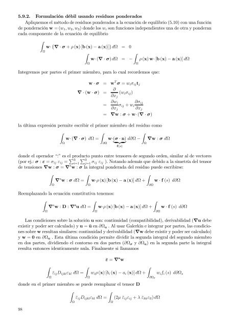
5.9.2. Formulación débil usando <strong>residuos</strong> pon<strong>de</strong>rados<br />
Apliquemos el método <strong>de</strong> <strong>residuos</strong> pon<strong>de</strong>rados a la ecuación <strong>de</strong> equilibrio (5.10) con una función<br />
<strong>de</strong> pon<strong>de</strong>ración w = (w 1 , w 2 , w 3 ) don<strong>de</strong> los w i son funciones in<strong>de</strong>pendientes una <strong>de</strong> otra y pon<strong>de</strong>ran<br />
cada componente <strong>de</strong> la ecuación <strong>de</strong> equilibrio<br />
∫<br />
Ω<br />
w· {∇ · σ + ρ (x) [b (x) − a (x)]} dΩ = 0<br />
∫<br />
∫<br />
w· (∇ · σ) dΩ = −<br />
Ω<br />
Integremos por partes el primer miembro, para lo cual recor<strong>de</strong>mos que:<br />
Ω<br />
ρ (x) w· [b (x) − a (x)] dΩ<br />
w · σ = w T σ = w i σ ij t j<br />
∇ · (w · σ) = ∂<br />
∂x j<br />
(w i σ ij )<br />
= ∂w i ∂σ ij<br />
σ ij + w i<br />
∂x j ∂x j<br />
= ∇w : σ + w· (∇ · σ)<br />
la última expresión permite escribir el primer miembro <strong>de</strong>l residuo como<br />
∫<br />
Ω<br />
∫<br />
w· (∇ · σ) dΩ =<br />
∂Ω<br />
∫<br />
w·(σ · n) d∂Ω − ∇w : σ dΩ<br />
} {{ }<br />
Ω<br />
f(s)<br />
don<strong>de</strong> el operador “:” es el producto punto entre tensores <strong>de</strong> segundo or<strong>de</strong>n, similar al <strong>de</strong> vectores<br />
(por ej.: σ : ε = σ ij ε ij = ∑ 3<br />
∑ 3<br />
i=1 j=1 σ ij ε ij ). Notando a<strong>de</strong>más que <strong>de</strong>bido a la simetría <strong>de</strong>l tensor<br />
<strong>de</strong> tensiones ∇w : σ = ∇ s w : σ la integral pon<strong>de</strong>rada <strong>de</strong>l residuo pue<strong>de</strong> escribirse:<br />
∫<br />
Ω<br />
∫<br />
∇ s w : σ dΩ =<br />
Reemplazando la ecuación constitutiva tenemos:<br />
∫<br />
Ω<br />
∫<br />
∇ s w : D : ∇ s u dΩ =<br />
Ω<br />
∫<br />
w·ρ (x) [b (x) − a (x)] dΩ +<br />
Ω<br />
∂Ω<br />
∫<br />
w·ρ (x) [b (x) − a (x)] dΩ +<br />
w · f (s) d∂Ω<br />
∂Ω<br />
w · f (s) d∂Ω<br />
Las condiciones sobre la solución u son: continuidad (compatibilidad), <strong>de</strong>rivabilidad (∇u <strong>de</strong>be<br />
existir y po<strong>de</strong>r ser calculado) y u = ū en ∂Ω u . Al usar Galerkin e integrar por partes, las condiciones<br />
sobre w resultan similares: continuidad y <strong>de</strong>rivabilidad (∇w <strong>de</strong>be existir y po<strong>de</strong>r ser calculado)<br />
y w = 0 en ∂Ω u . Esta última condición permite dividir la segunda integral <strong>de</strong>l segundo miembro<br />
en dos partes, dividiendo el contorno en dos partes (∂Ω σ y ∂Ω u ) en la segunda parte la integral<br />
resulta entonces i<strong>de</strong>nticamente nula. Finalmente si llamamos<br />
∫<br />
Ω<br />
∫<br />
¯ε ij D ijkl ε kl dΩ =<br />
Ω<br />
¯ε = ∇ s w<br />
∫<br />
w i ρ (x) [b i (x) − a i (x)] dΩ + w i f i (s) d∂Ω s<br />
∂Ω σ<br />
don<strong>de</strong> en el primer miembro se pue<strong>de</strong> reemplazar el tensor D<br />
98<br />
∫<br />
Ω<br />
∫<br />
¯ε ij D ijkl ε kl dΩ =<br />
Ω<br />
(2µ ¯ε ij ε ij + λ ¯ε kk ε ll ) dΩ