Capítulo 1 Métodos de residuos ponderados Funciones de prueba ...
Capítulo 1 Métodos de residuos ponderados Funciones de prueba ...
Capítulo 1 Métodos de residuos ponderados Funciones de prueba ...

You also want an ePaper? Increase the reach of your titles
YUMPU automatically turns print PDFs into web optimized ePapers that Google loves.
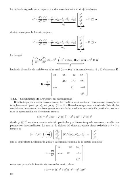
La <strong>de</strong>rivada segunda <strong>de</strong> u respecto a x dos veces (curvatura <strong>de</strong>l eje medio) es<br />
⎡ ⎤<br />
u 1<br />
u ′′ = d2 u d 2 ξ<br />
dξ 2 dx = 4 [ ]<br />
φ<br />
1 2 L 2 ′ ξξ, ϕ 1′ ξξ, φ 2′ ξξ, ϕ 2′ ⎢ β 1<br />
⎥<br />
ξξ ⎣<br />
} {{ }<br />
u 2 ⎦ = B (ξ) u<br />
B(ξ)<br />
β 2<br />
} {{ }<br />
u<br />
similarmente para la función <strong>de</strong> peso<br />
La integral<br />
∫<br />
v ′′ = d2 v<br />
dξ 2 d 2 ξ<br />
L<br />
dx = 4 [<br />
φ<br />
1 2 L 2 ′ ξξ, ϕ 1′ ξξ, φ 2′ ξξ, ϕ 2′ ξξ<br />
} {{ }<br />
B(ξ)<br />
]<br />
⎡ ⎤<br />
v 1<br />
⎢ θ 1<br />
⎥<br />
⎣ v 2 ⎦<br />
θ 2<br />
} {{ }<br />
v<br />
= B (ξ) v<br />
d 2 v<br />
dx EI d2 u<br />
2 dx<br />
∫L<br />
dx = 2 vT B T (ξ) (EI) B (ξ) dx u = v T K u<br />
} {{ }<br />
K<br />
haciendo el cambio <strong>de</strong> variable en la integral (dx = L dξ e integrando entre -1 y 1) obtenemos K<br />
2<br />
⎡<br />
⎤<br />
12 6L −12 6L<br />
K = EI<br />
4L 2 −6L 2L 2<br />
L 3 ⎢ sim. 12 −6L<br />
⎥<br />
⎣<br />
⎦<br />
4L 2<br />
4.3.1. Condiciones <strong>de</strong> Dirichlet no-homogéneas<br />
Resulta importante notar como se tratan las condiciones <strong>de</strong> contorno esenciales no homogéneas<br />
(<strong>de</strong>splazamiento prescriptos), sea por ej. (β 1 = ¯β 1 ). Recor<strong>de</strong>mos que en el método <strong>de</strong> Galerkin las<br />
condiciones <strong>de</strong> contorno no homogéneas se satisfacían mediante una solución particular, en este<br />
caso la aproximación en el elemento resulta<br />
u (ξ) = φ 1 (ξ) u 1 + ϕ 1 (ξ) ¯β 1 + φ 2 (ξ) u 2 + ϕ 2 (ξ) β 2<br />
don<strong>de</strong> ϕ 1 (ξ) ¯β 1 es ahora nuestra solución particular y el elemento queda entonces con sólo tres<br />
parámetros in<strong>de</strong>pendientes. La matriz <strong>de</strong> rigi<strong>de</strong>z <strong>de</strong>l elemento queda ahora reducida a 3 × 3 y<br />
resulta <strong>de</strong><br />
[ v 1 , v 2 , θ 2] ∫ ( ) ⎡ ⎤<br />
⎡ ⎤<br />
φ<br />
16<br />
1′ ξξ<br />
⎣ φ 2′ ⎦<br />
L 4 ξξ (EJ) [ ]<br />
u 1<br />
φ 1′ ξξ, φ 2′ ξξ, ϕ 2′ ξξ dx ⎣ u 2 ⎦<br />
ϕ 2′ ξξ<br />
β 2<br />
que es equivalente a eliminar la 2 fila y la segunda columna <strong>de</strong> la matriz completa<br />
⎡<br />
⎤<br />
12 −12 6L<br />
K = EI<br />
L 3 ⎢ sim. 12 −6L<br />
⎥<br />
⎣<br />
⎦<br />
4L 2<br />
notar que para ello la función <strong>de</strong> peso se ha escrito ahora<br />
62<br />
v (ξ) = φ 1 (ξ) v 1 + φ 2 (ξ) v 2 + ϕ 2 (ξ) θ 2