Capítulo 1 Métodos de residuos ponderados Funciones de prueba ...

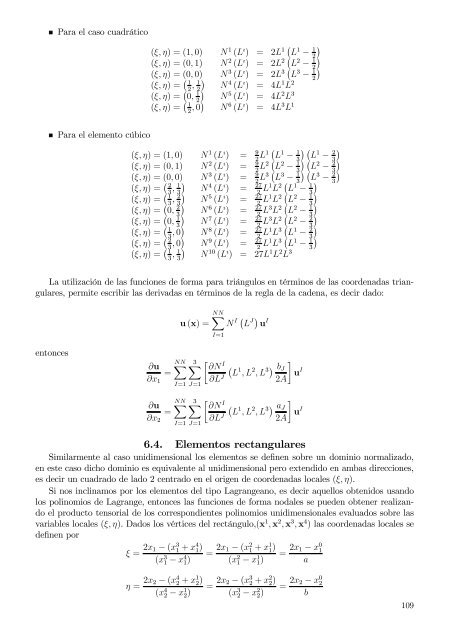
Para el caso cuadrático
(ξ, η) = (1, 0) N 1 (L ı ) = 2L ( )
1 L 1 − 1 2
(ξ, η) = (0, 1) N 2 (L ı ) = 2L ( )
2 L 2 − 1 2
(ξ, η) = (0, 0) N 3 (L ı ) = 2L ( )
3 L 3 − 1 2
(ξ, η) = ( 1
, )
1 N 4 (L ı ) = 4L 1 L 2
2 2
(ξ, η) = ( )
0, 1 N 5 (L ı ) = 4L 2 L 3
2
(ξ, η) = ( 1
, 0) N 6 (L ı ) = 4L 3 L 1
2
Para el elemento cúbico
(ξ, η) = (1, 0) N 1 (L ı ) = ( ( )
9
2 L1 L 1 − 3) 1 L 1 − 2 3
(ξ, η) = (0, 1) N 2 (L ı ) = ( ( )
9
2 L2 L 2 − 3) 1 L 2 − 2 3
(ξ, η) = (0, 0) N 3 (L ı ) = ( ( )
9
2 L3 L 3 − 3) 1 L 3 − 2 3
(ξ, η) = ( 2
, )
1 N 4 (L ı ) = 27 3 3
2 L1 L ( )
2 L 1 − 1 3
(ξ, η) = ( 1
, )
2 N 5 (L ı ) = 27 3 3
2 L1 L ( )
2 L 2 − 1 3
(ξ, η) = ( )
0, 2 N 6 (L ı ) = 27 3
2 L3 L ( )
2 L 2 − 1 3
(ξ, η) = ( )
0, 1 N 7 (L ı ) = 27 3
2 L3 L ( )
2 L 2 − 2 3
(ξ, η) = ( 1
3 , 0) N 8 (L ı ) = 27 2 L1 L ( )
3 L 1 − 2 3
(ξ, η) = ( 2
, 0) N 9 (L ı ) = 27 3 2 L1 L ( )
3 L 1 − 1 3
(ξ, η) = ( 1
, )
1 N 10 (L ı ) = 27L 1 L 2 L 3
3 3
La utilización de las funciones de forma para triángulos en términos de las coordenadas triangulares,
permite escribir las derivadas en términos de la regla de la cadena, es decir dado:
u (x) =
NN∑
I=1
N I ( L J) u I
entonces
∂u
NN∑
=
∂x 1
I=1 J=1
∂u
NN∑
=
∂x 2
I=1 J=1
3∑
[ ∂N
I
3∑
[ ∂N
I
∂L J (
L 1 , L 2 , L 3) b J
2A
∂L J (
L 1 , L 2 , L 3) a J
2A
]
u I
]
u I
6.4. Elementos rectangulares
Similarmente al caso unidimensional los elementos se definen sobre un dominio normalizado,
en este caso dicho dominio es equivalente al unidimensional pero extendido en ambas direcciones,
es decir un cuadrado de lado 2 centrado en el origen de coordenadas locales (ξ, η).
Si nos inclinamos por los elementos del tipo Lagrangeano, es decir aquellos obtenidos usando
los polinomios de Lagrange, entonces las funciones de forma nodales se pueden obtener realizando
el producto tensorial de los correspondientes polinomios unidimensionales evaluados sobre las
variables locales (ξ, η). Dados los vértices del rectángulo,(x 1 , x 2 , x 3 , x 4 ) las coordenadas locales se
definen por
ξ = 2x 1 − (x 3 1 + x4 1 )
(x 3 1 − x 4 1)
= 2x 1 − (x 2 1 + x1 1 )
(x 2 1 − x 1 1)
= 2x 1 − x 0 1
a
η = 2x 2 − (x 4 2 + x1 2 )
(x 4 2 − x 1 2)
= 2x 2 − (x 3 2 + x2 2 )
(x 3 2 − x 2 2)
= 2x 2 − x 0 2
b
109