Capítulo 1 Métodos de residuos ponderados Funciones de prueba ...

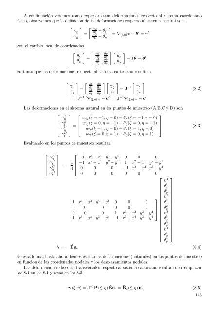
A continuación veremos como expresar estas deformaciones respecto al sistema coordenado
físico, observemos que la definición de las deformaciones respecto al sistema natural son:
[ ] [ ∂w
γξ
=
− θ ]
∂ξ ξ
∂w
γ η ∂η − θ = ∇ (ξ,η) w − θ ′ = γ ′
η
con el cambio local de coordenadas
[ ]
θξ
=
θ η
[
∂x
∂ξ
∂x
∂η
∂y
∂ξ
∂y
∂η
] [ ]
θx
= Jθ = θ ′
θ y
en tanto que las deformaciones respecto al sistema cartesiano resultan:
[
γx
]
=
γ y
[ ∂ξ
∂x
∂ξ
∂y
∂η
∂x
∂η
∂y
] [
γξ
γ η
]
= J −1 [
γξ
γ η
]
= J −1 [ ∇ (ξ,η) w − θ ′] = J −1 ∇ (ξ,η) w − θ
(8.2)
Las deformaciones en el sistema natural en los puntos de muestreo (A,B,C y D) son
⎡ ⎤ ⎡
⎤
γ A η
w′ ⎢ γ B η (ξ = −1, η = 0) − θ η (ξ = −1, η = 0)
ξ ⎥
⎣ γ C ⎦ = ⎢
w′ ξ (ξ = 0, η = −1) − θ ξ (ξ = 0, η = −1)
⎥
⎣
η
w′ η (ξ = 1, η = 0) − θ η (ξ = 1, η = 0) ⎦ (8.3)
γ D ξ
w′ ξ (ξ = 0, η = 1) − θ ξ (ξ = 0, η = 1)
Evaluando en los puntos de muestreo resultan
⎡
⎢
⎣
γ A η
γ B ξ
γ C η
γ D ξ
⎤
⎥
⎦ = 1 4
⎡
⎢
⎣
−1 x 4 − x 1 y 4 − y 1 0 0 0
−1 x 2 − x 1 y 2 − y 1 1 x 2 − x 1 y 2 − y 1
0 0 0 −1 x 3 − x 2 y 3 − y 2
0 0 0 0 0 0
⎤
1 x 4 − x 1 y 4 − y 1 0 0 0
0 0 0 0 0 0
⎥
0 0 0 1 x 3 − x 2 y 3 − y 2 ⎦
1 x 3 − x 4 y 3 − y 4 −1 x 3 − x 4 y 3 − y 4 ⎢
⎣
ˆγ = ˆBu e (8.4)
⎡
w 1
θ 1 x
θ 1 y
w 2
θ 2 x
θ 2 y
w 3
θ 3 x
θ 3 y
w 4
θ 4 x
θ 4 y
⎤
⎥
⎦
de esta forma, hasta ahora, hemos escrito las deformaciones (naturales) en los puntos de muestreo
en función de las coordenadas nodales y los desplazamientos nodales.
Las deformaciones de corte transversales respecto al sistema cartesiano resultan de reemplazar
las 8.4 en las 8.1 y estas en las 8.2
γ (ξ, η) = J −1 P (ξ, η) ˆBu e = ¯B s (ξ, η) u e (8.5)
145