Capítulo 1 Métodos de residuos ponderados Funciones de prueba ...

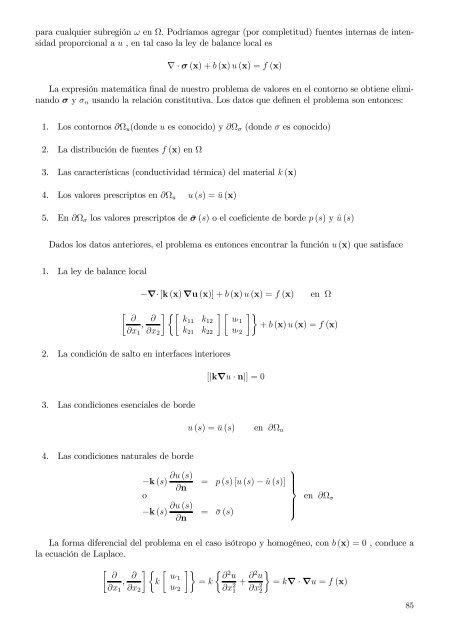
para cualquier subregión ω en Ω. Podríamos agregar (por completitud) fuentes internas de intensidad
proporcional a u , en tal caso la ley de balance local es
∇ · σ (x) + b (x) u (x) = f (x)
La expresión matemática final de nuestro problema de valores en el contorno se obtiene eliminando
σ y σ n usando la relación constitutiva. Los datos que definen el problema son entonces:
1. Los contornos ∂Ω u (donde u es conocido) y ∂Ω σ (donde σ es conocido)
2. La distribución de fuentes f (x) en Ω
3. Las características (conductividad térmica) del material k (x)
4. Los valores prescriptos en ∂Ω u u (s) = ū (x)
5. En ∂Ω σ los valores prescriptos de ¯σ (s) o el coeficiente de borde p (s) y û (s)
Dados los datos anteriores, el problema es entonces encontrar la función u (x) que satisface
1. La ley de balance local
−∇· [k (x) ∇u (x)] + b (x) u (x) = f (x)
en Ω
[ ] {[ ] [ ∂ ∂ k11 k
,
12 u′ 1
∂x 1 ∂x 2 k 21 k 22 u′ 2
2. La condición de salto en interfaces interiores
[|k∇u · n|] = 0
]}
+ b (x) u (x) = f (x)
3. Las condiciones esenciales de borde
u (s) = ū (s)
en ∂Ω u
4. Las condiciones naturales de borde
−k (s)
o
−k (s)
∂u (s)
∂n
∂u (s)
∂n
= p (s) [u (s) − û (s)]
= ¯σ (s)
⎫
⎪⎬
⎪⎭
en ∂Ω σ
La forma diferencial del problema en el caso isótropo y homogéneo, con b (x) = 0 , conduce a
la ecuación de Laplace.
[ ] { [ ∂ ∂ u′ 1
, k
∂x 1 ∂x 2 u′ 2
]}
{ ∂ 2 u
= k
∂x 2 1
}
+ ∂2 u
= k∇ · ∇u = f (x)
∂x 2 2
85