Capítulo 1 Métodos de residuos ponderados Funciones de prueba ...

[ ]
N
1
′ x
−N
[B s ] 2×12
=
1 0 N 2
′ x
−N 2 0 N 3
′ x
−N 3 0 N 4
′ x
−N 4 0
N 1
′ y 0 −N 1 N 2
′ y 0 −N 2 N 3
′ y 0 −N 3 N 4
′ y 0 −N 4
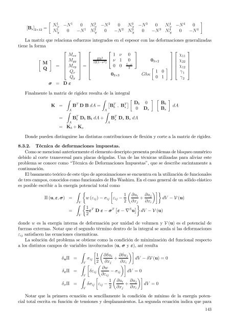
La matriz que relaciona esfuerzos integrados en el espesor con las deformaciones generalizadas
tiene la forma
⎡ ⎤ ⎡ ⎡
⎤
⎤ ⎡ ⎤
M xx
1 ν 0
χ 11
[ ]
M M yy
Eh =
Q ⎢ M xy
⎥
⎣ Q x
⎦ = 3
⎣ ν 1 0 ⎦ 0
12(1−ν 2 )
3×2
χ 22
⎢ 0 0 1−ν
2 [ ] ⎥ ⎢ χ 12
⎥
⎣
1 0 ⎦ ⎣ γ
0
Q 2×3 Ghκ
1
⎦
y
0 1 γ 2
σ = D ε
Finalmente la matriz de rigidez resulta de la integral
∫
∫
[ ] [ ] [ ]
K = B T D B dA = B
T
b , B T D b 0 Bb
s
dA
A
A
0 D s B s
∫
∫
= B T b D b B b dA + B T s D s B s dA
A
= K b + K s
A
Donde pueden distinguirse las distintas contribuciones de flexión y corte a la matriz de rigidez.
8.3.2. Técnica de deformaciones impuestas.
Como se mencionó anteriormente el elemento descripto presenta problemas de bloqueo numérico
debido al corte transversal para placas delgadas. Una de las técnicas utilizadas para aliviar este
problema se conoce como “Técnica de Deformaciones Impuestas”, que se describe sucintamente a
continuación.
El basamento teórico de este tipo de aproximaciones se encuentra en la utilización de funcionales
de tres campos, conocidos como funcionales de Hu-Washizu. En el caso general de un sólido elástico
es posible escribir a la energía potencial total como
∫
[
Π (u, ε, σ) =
{w (ε ij ) − σ ij ε ij − 1 ( ∂ui
+ ∂u )]}
j
dV − V (u)
V
2 ∂x j ∂x i
∫ { 1
=
2 εT D ε − σ [ T ε − ∇ S u ]} dV − V (u)
V
donde w es la energía interna de deformación por unidad de volumen y V (u) es el potencial de
fuerzas externas. Notar que el segundo término dentro de la integral se anula si las deformaciones
ε ij satisfacen las ecuaciones cinemáticas.
La solución del problema se obtiene como la condición de minimización del funcional respecto
a los distintos campos de variables involucrados (u, σ y ε), así resulta
δ u Π =
δ ε Π =
δ σ Π =
∫
∫
∫
V
V
V
( ∂δui
[ 1
σ ij
2 ∂x j
[ ( )]
∂w
δε ij − σ ij
∂ε ij
δσ ij
[
ε ij − 1 2
+ ∂δu j
∂x i
)]
dV − δV (u) = 0
dV = 0
( ∂ui
+ ∂u )]
j
dV = 0
∂x j ∂x i
Notar que la primera ecuación es sencillamente la condición de mínimo de la energía potencial
total escrita en función de tensiones y desplazamientos. La segunda ecuación indica que para
143