Capítulo 1 Métodos de residuos ponderados Funciones de prueba ...

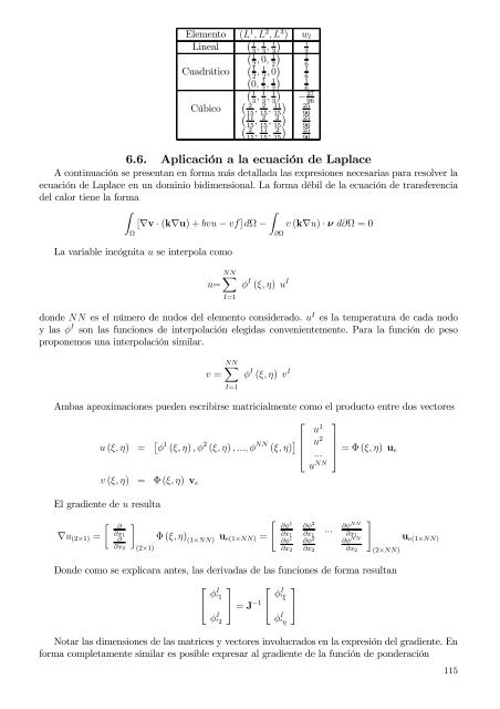
Elemento (L
( 1 , L 2 , L 3 ) w l
Lineal 1 , 1, 1 1
( 3 3 3)
2
1 , 0, 1 1
( 2 2)
6
Cuadrático 1 , 1, 0) 1
( 2 2 6
0,
1
, )
1 1
( 2 2 6
1
( 3 , 1 3 , 3)
1 − 27
96
Cúbico 2
15 , 2
15 , )
11 25
( 15 96
11
15 , 2
15 , )
2 25
( 15 96
2
15 , 11
15 , )
2 25
15 96
6.6. Aplicación a la ecuación de Laplace
A continuación se presentan en forma más detallada las expresiones necesarias para resolver la
ecuación de Laplace en un dominio bidimensional. La forma débil de la ecuación de transferencia
del calor tiene la forma
∫
∫
[∇v · (k∇u) + bvu − vf] dΩ −
Ω
La variable incógnita u se interpola como
∂Ω
v (k∇u) · ν d∂Ω = 0
u=
NN∑
I=1
φ I (ξ, η) u I
donde NN es el número de nudos del elemento considerado. u I es la temperatura de cada nodo
y las φ I son las funciones de interpolación elegidas convenientemente. Para la función de peso
proponemos una interpolación similar.
v =
NN∑
I=1
φ I (ξ, η) v I
Ambas aproximaciones pueden escribirse matricialmente como el producto entre dos vectores
u (ξ, η) = [ φ 1 (ξ, η) , φ 2 (ξ, η) , ..., φ NN (ξ, η) ] ⎡
v (ξ, η) = Φ (ξ, η) v e
El gradiente de u resulta
⎢
⎣
u 1
u 2
...
u NN
⎤
⎥
⎦ = Φ (ξ, η) u e
∇u (2×1) =
[ ∂
∂x 1
∂ Φ (ξ, η) (1×NN)
u e(1×NN) =
∂x 2
](2×1)
[
∂φ
1
∂φ 2
∂x ∂φ 1 ∂φ 2
∂x 2 ∂x 2
∂x 1
...
∂φ NN
∂x 1
u
∂φ NN
e(1×NN)
∂x 2
](2×NN)
Donde como se explicara antes, las derivadas de las funciones de forma resultan
⎡
⎣ φI′ 1
⎤ ⎡
⎦ = J −1 ⎣
φ I′ ξ
⎤
⎦
φ I′ 2
φ I′ η
Notar las dimensiones de las matrices y vectores involucrados en la expresión del gradiente. En
forma completamente similar es posible expresar al gradiente de la función de ponderación
115