Capítulo 1 Métodos de residuos ponderados Funciones de prueba ...
Capítulo 1 Métodos de residuos ponderados Funciones de prueba ...
Capítulo 1 Métodos de residuos ponderados Funciones de prueba ...

Create successful ePaper yourself
Turn your PDF publications into a flip-book with our unique Google optimized e-Paper software.
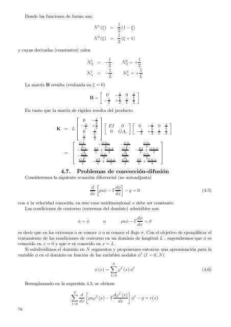
Don<strong>de</strong> las funciones <strong>de</strong> forma son:<br />
N 1 (ξ) = 1 (1 − ξ)<br />
2<br />
N 2 (ξ) = 1 (ξ + 1)<br />
2<br />
y cuyas <strong>de</strong>rivadas (constantes) valen<br />
N 1<br />
′ ξ = − 1 2<br />
N 1<br />
′ x = − 1 L<br />
N 2<br />
′ ξ = +1 2<br />
N 2<br />
′ x = + 1 L<br />
La matriz B resulta (evaluada en ξ = 0)<br />
[ 0 −<br />
1<br />
B =<br />
− 1 + 1 L 2<br />
1<br />
0<br />
L L<br />
1 1<br />
L 2<br />
]<br />
En tanto que la matriz <strong>de</strong> rigi<strong>de</strong>z resulta <strong>de</strong>l producto<br />
⎡ ⎤<br />
0 − 1 L [ ] [ K = L ⎢ − 1 + 1 L 2 ⎥ EI 0 0 −<br />
1<br />
⎣ 1<br />
0 ⎦ 0 GA<br />
L<br />
c − 1 + 1 L 2<br />
=<br />
⎡<br />
⎢<br />
⎣<br />
1<br />
L<br />
GA c<br />
L<br />
− GAc<br />
2<br />
− GAc<br />
L<br />
1<br />
2<br />
GA c<br />
− EI<br />
2 L<br />
1<br />
0<br />
L L<br />
1 1<br />
L 2<br />
− GA 0c<br />
− GA c GA c<br />
2 L<br />
2<br />
EI<br />
+ GAcL GA c<br />
− EI + GAcL<br />
L 2 2 L 2<br />
GA c GA c GA c<br />
+<br />
2<br />
GA L<br />
2<br />
cL GA c EI<br />
2 2 L<br />
+ GA cL<br />
2<br />
4.7. Problemas <strong>de</strong> convección-difusión<br />
Consi<strong>de</strong>remos la siguiente ecuación diferencial (no autoadjunta)<br />
[<br />
d<br />
ρuφ − Γ dφ ]<br />
− q = 0 (4.5)<br />
dx dx<br />
con u la velocidad conocida, en este caso unidimensional u <strong>de</strong>be ser constante.<br />
Las condiciones <strong>de</strong> contorno (extremos <strong>de</strong>l dominio) admisibles son:<br />
φ = ¯φ o ρuφ − Γ dφ<br />
dx = ¯σ<br />
es <strong>de</strong>cir que en los extremos o se conoce φ o se conoce el flujo σ. Con el objetivo <strong>de</strong> ejemplificar el<br />
tratamiento <strong>de</strong> las condiciones <strong>de</strong> contorno en un dominio <strong>de</strong> longitud L , supondremos que φ es<br />
conocido en x = 0 y que σ es conocido en x = L.<br />
Si subdividimos el dominio en N segmentos y proponemos entonces una aproximación para la<br />
variable φ en el dominio en función <strong>de</strong> las variables nodales φ I (I = 0..N)<br />
⎤<br />
⎥<br />
⎦<br />
]<br />
φ (x) =<br />
N∑<br />
ϕ I (x) φ I (4.6)<br />
I=0<br />
78<br />
Reemplazando en la expresión 4.5, se obtiene<br />
N∑<br />
I=0<br />
[<br />
]<br />
d<br />
ρuϕ I (x) − Γ dϕI (x)<br />
φ I − q = r(x)<br />
dx<br />
dx