Capítulo 1 Métodos de residuos ponderados Funciones de prueba ...
Capítulo 1 Métodos de residuos ponderados Funciones de prueba ...
Capítulo 1 Métodos de residuos ponderados Funciones de prueba ...

Create successful ePaper yourself
Turn your PDF publications into a flip-book with our unique Google optimized e-Paper software.
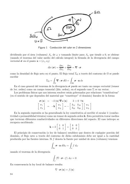
Figura 1<br />
Conducción <strong>de</strong>l calor en 2 dimensiones<br />
dividiendo por el área (volumen) A ω <strong>de</strong> ω y tomando límite para A ω que tien<strong>de</strong> a 0, se obtiene<br />
(usando el teorema <strong>de</strong>l valor medio <strong>de</strong>l cálculo integral) la fórmula <strong>de</strong> la divergencia <strong>de</strong>l campo<br />
vectorial σ en el punto x = (x 1 , x 2 )<br />
div (σ) = ∂σ 1<br />
∂x 1<br />
+ ∂σ 2<br />
∂x 2<br />
= ∇ · σ<br />
como la <strong>de</strong>nsidad <strong>de</strong> flujo neto en el punto. El flujo total Σ Ω a través <strong>de</strong>l contorno <strong>de</strong> Ω se pue<strong>de</strong><br />
escribir<br />
∫<br />
∫<br />
Σ Ω = ∇ · σ dΩ = σ · n ds<br />
Ω<br />
En el caso general <strong>de</strong>l teorema <strong>de</strong> la divergencia σ pue<strong>de</strong> ser tanto un campo vectorial (tensor<br />
<strong>de</strong> 1er. or<strong>de</strong>n) como un campo tensorial (2do. or<strong>de</strong>n), en el segundo caso Σ es un vector.<br />
Los problemas físicos que nos interesa resolver están gobernados por relaciones “constitutivas”<br />
(en el sentido <strong>de</strong> que <strong>de</strong>pen<strong>de</strong>n <strong>de</strong>l material que “constituye” el dominio) lineales <strong>de</strong> la forma<br />
σ (x) = −k (x) ∇u (x) k > 0 ∀x<br />
] [ ] [ ] [ ]<br />
u′ 1 k11 k<br />
= −k = −<br />
12 u′ 1<br />
σ 2 k 21 k 22<br />
[<br />
σ1<br />
u′ 2<br />
En la segunda expresión se ha generalizado la ley constitutiva al escribir el escalar k (conductividad<br />
o permeabilidad térmica) como un tensor <strong>de</strong> segundo or<strong>de</strong>n k. Esto permitiría tratar medios<br />
que tuvieran diferentes conductivida<strong>de</strong>s en diferentes direcciones <strong>de</strong>l espacio. El caso isótropo se<br />
recupera escribiendo<br />
[ 1 0<br />
k = k<br />
0 1<br />
]<br />
=<br />
∂Ω<br />
[ k 0<br />
0 k<br />
El principio <strong>de</strong> conservación (o ley <strong>de</strong> balance) establece que <strong>de</strong>ntro <strong>de</strong> cualquier porción <strong>de</strong>l<br />
dominio, el flujo neto a través <strong>de</strong>l contorno <strong>de</strong> dicho subdominio <strong>de</strong>be ser igual a la cantidad<br />
producida por las fuentes internas. Si f <strong>de</strong>nota la fuente por unidad <strong>de</strong> área (volumen) tenemos<br />
∫<br />
∫<br />
σ · n d∂ω = f dω<br />
usando el teorema <strong>de</strong> la divergencia<br />
En consecuencia la ley local <strong>de</strong> balance resulta<br />
∂ω<br />
∫<br />
ω<br />
ω<br />
(∇ · σ−f) dω = 0<br />
]<br />
u′ 2<br />
84<br />
∇ · σ (x) = f (x)