Online proceedings - EDA Publishing Association

7-9 October 2009, Leuven, Belgium
For the simulation of global flow variables, the model from θ ( x)
and
s θ ( x)
are the non-dimensional solid and fluid
f
Bau is used, assuming fully developed laminar flow. This
temperatures; Nu ( α ) is the Nusselt number;
model calculates the non-dimensional mass flow rate m,
α
max
= maxα( x)
is
0≤x≤1
defined relative to the mass flow rate scale
* * * * *
m ( )
0
= hc Δp
ν L . the maximum aspect ratio of the channel; k s is the ratio
*
*
h is the channel’s height;
c
Δ p is the pressure drop over the
between the conductivity of solid and fluid k * s /k * f ; A s and A f
are the areas of the cross-sections of the solid and fluid
*
channels; ν is the kinematic viscosity of the coolant. The
*
region, non-dimensionalized with ( L ) 2
;
* * * *
χ = ( k
dimensionless mass flow m depends on the aspect ratio shape
f
L / c m
) with
0
profile
* *
α ( x ) = wc ( x) h c
along the channel:
c * the fluid heat capacity. The parameter χ is inverse
1
−1
*
proportional to
⎛ 1 (1 + α)²
⎞
Δ p .
m = ⎜ ( ) ⎟
8∫ Po α dx
(1)
³
The three terms in (3) represent respectively the heat
⎝ α
0 ⎠
source, the convective heat transfer from solid wall to the
*
Herein is Po (α ) the Poiseuille number and x = x * L is the coolant and axial conductive heat transfer in the solid wall.
In these equations –using
*'' * *
Q s
hc
k III. OPTIMIZATION PROCEDURE
f
The shape of the channels is optimized with respect to two
dimensionless axial coordinate. For the determination of the
Poiseuille number, following correlation for fully developed
flow is used [10] ( 0 ≤ α ≤1):
Similarly, the three terms in (4) represent convective heat
transfer from solid to coolant, the axial conductive heat
transfer in the coolant and the capacitive heating of the fluid.
2
3
Po ( α ) = 96(1 −1.3553α
+ 1.9467α
−1.7012α
(2)
A constant heat flux correlation for Nu ( α ) is used in the
4
5
+ 0.9564α
− 0.2537α
).
assumption of fully developed flow with three-wall heating
The simulation of the axial temperature profiles introduces [10] ( 0 ≤ α ≤1):
2
3
some differences with the model from Bau. In this model, Nu ( α ) = 8.235(1 −1.883α
+ 3.767α
− 5.814α
(5)
axial temperature distribution is calculated for both the fluid
4 5
+ 5.361α
− 2α
).
and the solid wall region including axial conduction. The set of modeling equations (3)-(4) is solved numerically
Therefore, a set of 2 dimensionless heat transfer equations – using finite volume discretization with appropriate boundary
one for each region– is introduced.
conditions. The fluid inlet has a specified temperature. The
The equation describing heat transfer in the solid wall is:
Nu
( )
( α )( 1+
α )( 2 + α ) fluid outlet and both ends of the solid wall have adiabatic
d ⎛ dθ
s ⎞
α
max
+ w
f
−
⋅ ( θ
s
−θ
f
) + ⎜ks
As
⎟ = 0 boundary conditions.
2α
dx ⎝ dx ⎠
If the axial conduction terms in (3)-(4) are ignored, the
(3) modeling equations of Bau are retrieved. It is recalled in (6):
The heat transfer in the fluid region is described by:
Nu( α )( 1 + α )( 2 + α ) ⎛ 2α
χ ⎞
θ
d ⎛ dθ
f ⎞ m dθ
s
( x)
= ( α + w ) ⎜
+ ⋅ x⎟ (6)
max f
f
⋅ ( θ
s
−θ
f
) + ⎜ A ⎟
f
= ⋅ (4)
⎝ Nu( α )( 1+
α )( 2 + α ) m ⎠
2α
dx
dx
⎝ ⎠ χ dx
objectives. The first objective J consists of the
1
minimization of the wall temperature gradient. This is
formulated as the Euclidian norm of the local wall
temperature gradient dθ s
(x)
:
dx
2
⎛ ⎞
= 1 dθ
s
J ∫ ⎜ ⎟ ( ) 0
⎝ dx
dx
α x ⎠
(7)
The second objective J that is regarded is the
2
minimization of the thermal resistance, which is defined as
the maximum dimensionless wall temperature along the
channel:
J = min maxθ
( )
s
α ( x)
x
(8)
The primary variable describing the shape of the channels
is the aspect ratio profile α (x), which is a dimensionless
representation of the channel width. This shape profile is in
fact a continuous function defined over the entire length of
the channel. Conventional optimization routines are only
suitable for a finite number of variables. Therefore a
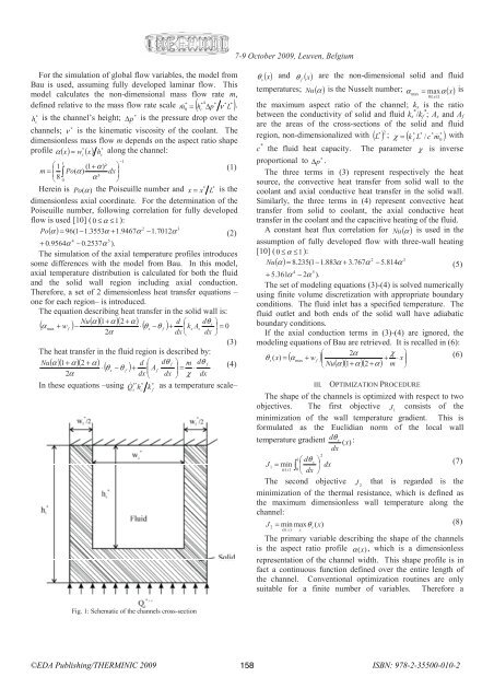
Fig. 1: Schematic of the channels cross-section
©EDA Publishing/THERMINIC 2009 158
ISBN: 978-2-35500-010-2