PRECIZIA ROBOŢILOR INDUSTRIALI

More documents

Recommendations

Info

Următoarele ecuaţii determinate prin identificarea termenilor corespunzători din matricele (3.65), respectiv (3.10) sunt utile în verificarea calculului erorilor unghiulare: i−1 nT i−1 r ⎧Δ ⎪ αz +Δ γ z= yi ⋅ xi ⎨ ⎪⎩ 1−Δα ⋅Δ γ = x ⋅ x i−1 nT i−1 r z z i i K. Determinarea erorilor unghiulare pentru setul de unghiuri ( αz−βy − γz) 109 ; (3.71) ⎡ 1 −Δαz 0⎤ ⎡ 1 0 Δβ 1 y ⎤ ⎡ 1 −Δγz 0⎤ ⎡ −Δγ z − Δαz Δβy⎤ ⎢ ⎢ ⎥ ⎢ ⎥ Δαz 1 0⎥⋅ 0 1 0 ⎢ γz 1 0⎥ Δ αz +Δγz 1 0 ⎢ ⎥ ⋅ Δ = ⎢ ⎥ (3.72) ⎢ ⎥ ⎢ ⎥ ⎢⎣ 0 0 1⎥⎦ ⎢−Δ ⎣ βy 0 1 ⎥⎦ ⎢⎣ 0 0 1⎥⎦ ⎢ −Δβy 0 1 ⎥ ⎣ ⎦ de unde se obţine: i−1 nT i−1 r y xi zi Δ β = ⋅ (3.73) i−1 nT i−1 r 1 i−1 nT i−1 r ( ) ( ), Δβ ⋅Δ α =− y ⋅ z ⇒ Δ α =− ⋅ y ⋅ z Δβ ≠ 0 y z i i z i i y Δβy i−1 nT i−1 r y i ⋅ zi z i−1 nT i−1 r xi ⋅ zi Δ α =− i−1 nT i−1 r 1 i−1 nT i−1 r Δβy ⋅Δ γ z = zi ⋅ y i ⇒ Δ γ z = ⋅( zi ⋅ y i ), Δβy ≠ 0 Δβ Din ecuaţia (3.73) se obţine valoarea erorii unghiulare Δ γ z , după cum rezultă din expresia de mai jos: i−1 nT i−1 r zi ⋅ y i z i−1 nT i−1 r xi ⋅ zi Δ γ = y . (3.74) (3.75) (3.76) ; (3.77) Următoarele ecuaţii determinate prin identificarea termenilor corespunzători din matricele (3.72), respectiv (3.10) sunt utile în verificarea calculului erorilor unghiulare: i−1 nT i−1 r ⎧Δ αz +Δ γz= yi ⋅ xi ⎪ ⎨ ⎪ ⎩1−Δα ⋅Δ γ = x ⋅ x i−1 nT i−1 r z z i i L. Determinarea erorilor unghiulare pentru setul de unghiuri ( α x −βy − γz) ; (3.78) ⎡1 0 0 ⎤ ⎡ 1 0 Δβ ⎤ ⎡ 1 −Δγ0⎤ ⎡ 1 −Δγ Δβ ⎤ y z z y ⎢ ⎥ ⎢ ⎥ z 0 1 0 ⎢ ⎥ ⎢ ⎥ 0 1 α γ z 1 0 Δγz 1 −Δα ⎢ −Δ ⎥⋅⎢ ⎥⋅ ⎢Δ⎥ = ⎢ x⎥ ⎢0 Δαz 1 ⎥ ⎢−Δβy 0 1 ⎥ ⎢ 0 0 1⎥ ⎢−Δβy Δαx 1 ⎥ ⎣ ⎦ ⎣ ⎦ ⎣ ⎦ ⎣ ⎦ Se identifică termenii din matricea (3.79) cu termenii corespunzători din matricea (3.10), astfel: (3.79)
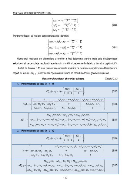
<strong>PRECIZIA</strong> ROBOȚILOR <strong>INDUSTRIALI</strong> . . ⎧Δ i−1 nT i−1 r α x = −( y i ⋅ zi ) ⎪ i−1 nT i−1 r ⎨Δ βy = xi ⋅ zi ; (3.80) ⎪ i−1 nT i−1 r ⎪⎩ Δ γ z =−( xi ⋅ yi ) Pentru verificare, se mai pot scrie următoarele identităţi: i−1 nT i−1 r ⎧Δ αx+Δβy ⋅Δ γz = zi ⋅ y i ⎪ i−1 nT i−1 r ⎨Δγ z ⋅Δαx −Δ βy = zi ⋅ xi (3.81) ⎪ i−1 nT i−1 r ⎪Δ ⎩ αx⋅Δ βy +Δ γz = y i ⋅ xi Operatorul matriceal de diferențiere a erorilor a fost determinat pentru toate cele douăsprezece seturi de matrice de rotație rezultantă, acestea din urmă fiind prezentate în detaliu și în cadrul capitolului 3. Astfel, în Tabelul 3.13 sunt prezentate expresiile analitice ce definesc operatorul de diferențiere în raport cu erorile δTii− 1 , echivalentul operatorului Uicker, în cadrul modelului geometric cu erori. 1. Pentru matricea de tipul (z – y – x) Operatorul matriceal al erorilor primare Tabelul 3.13 110 ( ψ ) ⎡ Δ × Δ pii −1 ⎤ δTii−1 ( z− y − x) = ⎢ ⎥ ⎢0 0 0 0 ⎥ ⎣ ⎦ ; (3.82) ⎡ 0 Δβy· sγ x −Δαz· cβy· cγ x Δ βy· cγ x +Δαz· cβy· sγ x⎤ ⎢ ⎥ Δ ( ψ × ) = ⎢ Δαz· cβy· cγ x −Δβy· sγ x 0 Δαz· sβy −Δγ x ⎥ ⎢ ⎥ ⎢−Δβy· cγ x −Δαz· cβy· sγ x Δγ x −Δαz· sβy 0 ⎣ ⎥⎦ ⎡ Δpx · cα 1 z· cβy −Δ pz · sβ · · 1 y +Δpy cβ 1 y sαz ⎤ ii− ii− ii− ⎢ ⎥ Δ p p ·( · · · ) ·( · · · ) · · 1 y cα 1 z cγ x sα ii ii z sβy sγ x px cγ ii 1 x sαz cαz sβy sγ x pz cβ ii 1 y sγ − = ⎢ Δ + −Δ − +Δ ⎥ x ⎢ − − − ⎥ ⎢Δ px ·( sα · c · · ) ·( · c · · ) · · ii 1 z sγ x + αz cγ x sβy −Δpy cα ii 1 z sγ x − γ x sαz sβy +Δpz cβ ii 1 y cγ⎥ ⎣ − − − x ⎦ 2. Pentru matricea de tipul (x – y – x) ( ψ ) ( ψ ) ⎡ Δ × Δ pii −1 ⎤ δTii−1 ( x− y − x) = ⎢ ⎥ ⎢0 0 0 0 ⎥ ⎣ ⎦ (3.83) (3.84) ; (3.85) ⎡ 0 Δβy· sγ x −Δαx· cγ x· sβy Δ βy· cγ x +Δαx· sβy· sγ x⎤ ⎢ ⎥ × =⎢ Δαx· cγ x· sβy −Δβy· sγ x 0 −Δγ x −Δαx· cβy ⎥ ; (3.86) ⎢ ⎥ ⎢⎣ −Δβy· cγ x − Δαx· sβy· sγ x Δ γ x + Δαx· cβy 0 ⎥⎦ ⎡ Δpx · cβ 1 y −Δ pz · cα · · · 1 x sβy +Δpy sα 1 x sβy ⎤ ii− ii− ii− ⎢ ⎥ Δ pii−1 = ⎢Δpy·( cα· · · ) ·( · · · ) · · ii 1 x cγ x − cβysαxsγ x +Δ pz cγ ii 1 x sαx+ cαxcβysγ x +Δpxsβ ii 1 y sγ x ⎥ − − − ⎢ ⎥ ⎢Δpx· cγ · ·( · · · ) ·( · · · ) ii 1 x sβy −Δpz sα ii 1 x sγ x −cαx cβy cγ x −Δ py cα ii 1 x sγ x + cβy cγ x sα − − − x ⎥ ⎣ ⎦ ;(3.87)
Page 1 and 2:
FACULTATEA CONSTRUCŢII DE MAŞINI
Page 3 and 4:
3. MODELAREA ERORILOR GEOMETRICE...
Page 5 and 6:
j { { i; j} = 1 → n } p ij , vect
Page 7 and 8:
{ unde i = 1 → n} qɺ i viteza li
Page 9 and 10:
xy Q Δ J Matricea Jacobiană pentr
Page 11 and 12:
NOȚIUNI GENERALE PRIVIND PRECIZIA
Page 13 and 14:
Page 15 and 16:
Page 17 and 18:
Page 19 and 20:
Page 21 and 22:
Page 23 and 24:
Page 25 and 26:
Page 27 and 28:
Page 29 and 30:
Page 31 and 32:
Page 33 and 34:
Page 35 and 36:
Page 37 and 38:
Page 39 and 40:
Page 41 and 42:
Page 43 and 44:
Page 45 and 46:
ALGORITMI DE CALCUL ÎN CINEMATICA
Page 47 and 48:
Page 49 and 50:
Page 51 and 52:
Page 53 and 54:
Page 55 and 56: ALGORITMI DE CALCUL ÎN CINEMATICA
Page 91 and 92: PRECIZIA ROBOȚILOR INDUSTRIALI . .
Page 105: PRECIZIA ROBOȚILOR INDUSTRIALI . .
Page 127 and 128: link i −1 q ⋅k i−1 i−1 { i
Page 129 and 130: 4.2 Matricea Jacobiană și proprie
Page 131 and 132: ( ) n0 X && t () 135 PRECIZIA ROBO
Page 133 and 134: 137 PRECIZIA ROBOȚILOR INDUSTRIALI
Page 139 and 140: 4.5 Matricea Jacobiană a erorilor
Page 141 and 142: 2 ( ) xek 0 J θ Δ & Q k=→ 1 n
Page 143 and 144: 2. im 0 i i i n ∑ k= i k−1 { (
Page 147 and 148: unde, [ ] T pk ε Di βi−1αi−1
Page 149 and 150: pk D unde, ε ∈ I11 , ceea ce în
Page 151 and 152: I69 . Se adoptă următoarele nota
Page 153 and 154: I ∗ Vectorii proprii ortonormali
Page 155 and 156: Ținând seama de faptul că N = 3
Page 157 and 158:
I111. Se notează cu Y = m ∑ k k
Page 159 and 160:
PRECIZIA ROBOȚILOR INDUSTRIALI Apl
Page 161 and 162:
6. MODELAREA ERORILOR DINAMICE 6.1
Page 163 and 164:
( ) ( C ) n n 0 ⎧ xy 0 0 xy xy
Page 165 and 166:
171 PRECIZIA ROBOȚILOR INDUSTRIALI
Page 167 and 168:
173 PRECIZIA ROBOȚILOR INDUSTRIALI
Page 169 and 170:
7. INFLUENȚA ERORILOR DINAMICE ASU
Page 171 and 172:
Prin aplicarea modelului direct al
Page 173 and 174:
q este un vector coloană m21 un ve
Page 175 and 176:
8.APLICAȚII PRIVIND DETERMINAREA P
Page 177 and 178:
APLICATII Matricea sistemelor de ti
Page 179 and 180:
3 4 APLICATII ⎡ 0. 77 ⎢ −0. 6
Page 181 and 182:
APLICATII Modulul erorilor vitezelo
Page 183 and 184:
APLICATII Robot M MD 6 R 15 25,2777
Page 185 and 186:
APLICATII Fig.8.4 Fig.8.5 Fig.8.6 1
Page 187 and 188:
APLICATII 192 Algoritmul matricei J
Page 189 and 190:
APLICATII 3 4 5 6 VD( t) OD( t) V(
Page 191 and 192:
APLICATII Cupla Matricea erorilor d
Page 193 and 194:
[C02] H.Chung, L. Ojeda, J. Borenst
Page 195 and 196:
[M07] Moorring, B.W, Roth, Z.S, Dri
Page 197:
[O01] L.Ojeda, L. Chung, H., and Bo
show all

PRECIZIA ROBOŢILOR INDUSTRIALI

Create successful ePaper yourself

Delete template?

Save as template?