PRECIZIA ROBOŢILOR INDUSTRIALI

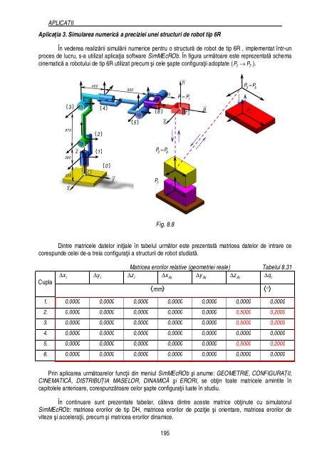
APLICATII
Aplicația 3. Simularea numerică a preciziei unei structuri de robot tip 6R
În vederea realizării simulării numerice pentru o structură de robot de tip 6R , implementat într-un
proces de lucru, s-a utilizat aplicaţia software SimMEcROb. În figura următoare este reprezentată schema
cinematică a robotului de tip 6R utilizat precum şi cele şapte configuraţii adoptate ( P1 → P7
).
Fig. 8.8
Dintre matricele datelor iniţiale în tabelul următor este prezentată matricea datelor de intrare ce
corespunde celei de-a treia configuraţii a structurii de robot studiată.
Cupla
{ }
3 { }
4
970
380
520
450
{ }
2
{ }
1
{ }
0
950
{ }
5
{ }
6
P2 = P6
P7
Matricea erorilor relative (geometriei reale) Tabelul 8.31
z
x
y
z
q Δ
Δ xi
i y Δ i Δ Δ Ai Δ Ai Δ Ai
i
mm °
1. 0,0000 0,0000 0,0000 0,0000 0,0000 0,0000 0,0000
2. 0,0000 0,0000 0,0000 0,0000 0,0000 0,5000 0,2000
3. 0,0000 0,0000 0,0000 0,0000 0,0000 0,5000 0,2000
4. 0,0000 0,0000 0,0000 0,0000 0,0000 0,0000 0,0000
5. 0,0000 0,0000 0,0000 0,0000 0,0000 0,5000 0,2000
6. 0,0000 0,0000 0,0000 0,0000 0,0000 0,0000 0,0000
620
Prin aplicarea următoarelor funcţii din meniul SimMEcROb şi anume: GEOMETRIE, CONFIGURAȚII,
CINEMATICĂ, DISTRIBUȚIA MASELOR, DINAMICĂ şi ERORI, se obţin toate matricele amintite în
capitolele anterioare, corespunzătoare celor şapte configuraţii luate în studiu.
În continuare sunt prezentate tabelar, câteva dintre aceste matrice obţinute cu simulatorul
SimMEcROb: matricea erorilor de tip DH, matricea erorilor de poziţie şi orientare, matricea erorilor de
viteze şi acceleraţii, precum şi matricea erorilor dinamice.
195
P = P1
{ }
7
P3 = P5
P4