commande optimale de l'alterno- demarreur avec prise en ... - UTC
commande optimale de l'alterno- demarreur avec prise en ... - UTC
commande optimale de l'alterno- demarreur avec prise en ... - UTC

You also want an ePaper? Increase the reach of your titles
YUMPU automatically turns print PDFs into web optimized ePapers that Google loves.
Tant que la vitesse reste nulle, voire très petite, l’expression (2.25) <strong>de</strong> la dynamique du<br />
courant statorique se réduit à la relation suivante :<br />
d I<br />
I s I mr + Tr.<br />
dt<br />
La solution particulière du courant magnétisant vaut :<br />
39<br />
mr<br />
= (2.29)<br />
= (2.30)<br />
I mrp ω<br />
K 2. exp( j.<br />
r.<br />
t)<br />
La solution générale du courant magnétisant <strong>de</strong> l’équation <strong>avec</strong> second membre <strong>de</strong>vi<strong>en</strong>t<br />
− t<br />
= K1.<br />
exp( ) + K 2.<br />
exp( j.<br />
r * . )<br />
(2.31)<br />
Tr<br />
Imr( t)<br />
ω t<br />
K2 s’obti<strong>en</strong>t <strong>en</strong> reportant la solution particulière dans l’équation différ<strong>en</strong>tielle :<br />
K 2<br />
K1 s’obti<strong>en</strong>t grâce aux conditions initiales<br />
d’où<br />
( ωr.<br />
Tr)<br />
Î Î mropt . 1+<br />
s<br />
=<br />
1+<br />
j.<br />
ω r.<br />
T 1+<br />
j.<br />
ωr.<br />
T<br />
= (2.32)<br />
− t<br />
( 0)<br />
= 0 = K1.<br />
exp( ) + K2.<br />
exp( j.<br />
r * . t)<br />
Tr<br />
Imr t<br />
ω<br />
= (2.33)<br />
K1 −K<br />
2<br />
²<br />
= (2.34)<br />
On obti<strong>en</strong>t finalem<strong>en</strong>t l’évolution temporelle du courant magnétisant :<br />
( ωr.<br />
Tr)<br />
1+<br />
² ⎡ − t ⎤<br />
= Î .<br />
.<br />
⎢<br />
exp( j.<br />
r * . t)<br />
− exp( )<br />
1+<br />
j.<br />
ωr.<br />
Tr<br />
⎥<br />
⎣<br />
Tr ⎦<br />
Imr( t)<br />
mropt<br />
ω<br />
On peut alors exprimer l’évolution temporelle du couple développé par le moteur :<br />
* { I s. I mropt }<br />
(2.35)<br />
3 Lm²<br />
C = . p.<br />
Im ag<br />
(2.36)<br />
2 Lr'