Esercizi e appunti per il corso di Fisica Matematica - Sezione di ...

More documents

Recommendations

Info

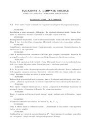
la struttura del ritratto di fase si cerca un integrale primo del sistema dinamico: si considera il campoν(x, y) = (4x(x 2 − 1), −2y) ortogonale in ogni punto al campo delle direzioni e, ricordando che l’integraleprimo deve avere gradiente parallelo a ν in ogni punto, deve esistere una funzione µ : R 2 → R tale che∇u(x, y) = µ(x, y)ν(x, y), ovvero∂u∂x = 4x(x2 − 1)µ(x, y)e∂u∂y= −2yµ(x, y) (2.19)Si deve determinare µ in modo che il campo differenziale costituito dalle due funzioni al secondo memebrodelle equazioni precedenti sia chiuso:∂∂y [4x(x2 − 1)µ(x, y)] = ∂∂x [−2yµ(x, y)] ⇒ [4x(x2 − 1)] ∂µ∂y = [−2y]∂µ ∂xL’equazione precedente è soddisfatta se si sceglie µ(x, y) = 1; allora l’integrale primo è soluzione delleequazioni (2.19) con µ = 1. Integrando la prima si ha u(x, y) = x 4 − 2x 2 + Φ(y), dove Φ è una funzionearbitraria della sola variabile y, sostituendo questa espressione nella seconda delle (2.19) si trovaΦ ′ (y) = −2y ⇒ Φ(y) = −y 2 + costante ⇒ u(x, y) = x 4 − 2x 2 − y 2 + 1 = (x 2 − 1) 2 − y 2dove la costante è stata scelta uguale a uno per porre u in una forma compatta. Si può verificare che icalcoli eseguiti sono corretti verificando che la derivata di Lie della funzione u rispetto al campo vettorialef è nulla in ongi punto:∇u · f = (4x 3 − 4x, −2y) · (2y, 4x 3 − 4x) = 8x 3 y − 8xy − 8x 3 y + 8xy = 0Per disegnare le curve di livello u(x, y) = a, con a ∈ R fissato, è conveniente iniziare con quelle passantiper i punti critici: u(−1, 0) = u(1, 0) = 0 e u(0, 0) = 1. Si considera dapprima la curva di livello a = 0,cioè (x 2 − 1) 2 − y 2 = 0, che fornisce le due parabole y = x 2 − 1 e y = −(x 2 − 1); quindi in corrispondenzadel valore a = 0 si hanno le due parabole passanti per i punti fissi P 1 e P 3 disegnate nel grafico di destradella figura 2.13. Si considera, ora, la curva di livello a = 1, cioè (x 2 − 1) 2 − 1 = y 2 , che fornisce ilpunto fisso nell’origine e le curve di equazione y = ± √ (x 2 − 1) 2 − 1 = ± √ x 2 (x 2 − 2). Queste curve sonodefinite nella regione x < √ 2 e x > √ 2, negli estremi degli intervalli di definizione intersecano l’asse y ein questo punto hanno derivata verticale, per esempio per il ramo positivod √x2 (xdx2 1− 2) =2 √ x 2 (x 2 − 2) (4x3 − 4x) = 2x(x2 − 1)√x2 (x 2 − 2)L’espressione della derivata appena calcolata mostra anche che l’arco di curva di livello considerato èdecrescente nella regione x < √ 2 e crescente nella regione x > √ 2. Tutte queste osservazioni permettonodi disegnare la curva di livello a = 1; si veda la figura 2.13.Tutte le altre curve di livello possono essere disegnate per continuità e il verso di percorrenza puòessere stabilito sulla base del campo delle direzioni sui punti della curva, si veda il grafico a destra nellafigura 2.13. Sulla base del ritratto di fase in figura si può concludere, anche se a rigore non si tratta didimostrazioni cristalline perché le linee di fase sono state dedotte con argomenti non del tutto rigorosi,che il punto fisso P 2 è stabile, mentre gli altri due punti fissi sono instabili. La curva di livello passanteper i punti fissi instabili, cioè la curva di livello u(x, y) = 0, è detta separatrice e in questo caso ècostitutita da due parabole.Per quanto riguarda i valori di a nelle diverse regioni in cui è suddiviso il ritratto di fase è sufficientecalcolare u(x, y) in qualche punto opportuno e poi ricordare che u è una funzione continua:– per a = 0, la curva di livello è la separatrice, cioè passa per i due punti fissi instabili, ed è costituitadall’unione dei due grafici delle parabole di equazione y = ±(x 2 − 1). Sulla separatrice giaccionootto linee di fase, due delle quali corrispondono ai punti fissi.fismat05.tex – 20 Aprile 2006 – 13:12 pagina 34
– Per a = 1, la curva di livello passa per il punto fisso stabile e consta di tre componenti conesse:una degenere e coicidente con l’origine e le altre due costituite dall’unione dei grafici delle funzioniy = ± √ x 2 (x 2 − 1) rispettivamente per x ≤ − √ 2 e x ≥ √ 2. Su ciascuna componente connessagiace una sola linea di fase, pertanto sulla curva di livello corrispondente ad a = 1 giacciono trelinee di fase.– Per a < 0, si hanno le curve di livello nella regione al di sopra delle separatrici e in quella al disotto delle separatrici; più precisamente ciascuna curva è costituita da due componenti connessele quali giacciono rispettivamente nelle regioni del piano delle fasiA a x 2 −1) o (−1 ≤ x ≤ 1 e y > 1−x 2 ) o (x ≥ 1 e y > x 2 −1)}eA a √ 2 e − √ x 2 (x 2 − 1) < y < √ x 2 (x 2 − 1)}A a>1,− := {(x, y) ∈ R 2 : x < − √ 2 e − √ x 2 (x 2 − 1) < y < √ x 2 (x 2 − 1)}Si noti che A a>1,− è ottenuta da A a>1,+ per simmetria rispetto all’asse y. Su ciascuna componenteconnessa di ciascuna curva di livello giace una sola linea di fase. Quindi su ciascuna curva di livellogiacciono due linee di fase.Le curve di livello u(x, y) = a sono equazioni algebriche di quarto grado che possono essere risolterispetto alla variabile y; per esempio il ramo positivo della curva di livello corrispondente ad a = 1 haequazione y = √ (x 2 − 1) 2 − 1. Questa proprietà permette di esprimere come integrale definito il tempodi percorrenza lungo l’orbita di fase, per esempio il tempo T che il sistema preparato nel punto ( √ 2, 0)impiega per giungere nel punto (2, 2 √ 2) si scrive come segue:ẋ = 2y ⇒ ẋ = 2 √ (x 2 − 1) 2 − 1 ⇒∫ 2√2∫dxT√(x2 − 1) 2 − 1 = 20dt ⇒ T = 1 2∫ 2√2dx√(x2 − 1) 2 − 1Questo integrale può essere calcolato numericamente o stimato con i metodi discussi nel paragrafo 1.4.Come secondo esempio si considera la separatrice y = −(x 2 − 1) e si suppone di preparare il sistemain (0, 1); sia T (b) il tempo impiegato per giungere in (b, 1 − b 2 ) con 0 ile 2006 – 13:12 pagina 35
Page 1 and 2: Esercizi e appunti per il corso di
Page 3 and 4: ⇒ x(t) = Ce tcon C ∈ RImpondend
Page 5 and 6: ✻x✟✻✟ ✟ ✟ ✟x✻x 0x
Page 7 and 8: viene scelto vicino a x 2 il sistem
Page 9 and 10: Esercizio 1.4. Supponendo uniforme
Page 11 and 12: Questo è parzialmente vero nel cas
Page 13 and 14: L’integrale, infatti, ha senso pe
Page 15 and 16: sensato, perché si ricorda che le
Page 17 and 18: dimostrare che il tempo t 1 − t 0
Page 19 and 20: con f : R n → R una funzione asse
Page 21 and 22: Come nel caso unidimensionale verif
Page 23 and 24: - asintoticamente stabile se e solo
Page 25 and 26: Esempio 2.9. Sulla base di argoment
Page 27 and 28: x 2✻✲✻ ✲✛ ✻❄✛ ❄
Page 29 and 30: Per esempio nel punto ¯x = (0, 1)
Page 31 and 32: livello chiusa, questa osservazione
Page 33: (x 2 + y 2 )/2. Si può verificare
Page 37 and 38: Teorema 2.21 Si consideri il sistem
Page 39 and 40: ciò fa intuire che in qualche sens
Page 41 and 42: Teorema 2.28 (Stabilità dei sistem
Page 43 and 44: La palla B δ (x e ) è proprio que
Page 45 and 46: e si studia la matrice associata al
Page 47 and 48: −ω 2 sin θ, dove ω = √ g/l
Page 49 and 50: Da questa proprietà segue che w è
Page 51 and 52: ✲✲✛✛P 3p✻✲✲✛✛P 2
Page 53 and 54: −πp✲✻✲✲ ✲✛0 π q✛
Page 55 and 56: è soddisfatta, perché L f ′w(q,
Page 57 and 58: y✻✛− √ 2✲✲ ✲✲✛
Page 59 and 60: Esercizio 2.16. Per i seguenti sist
Page 61 and 62: degli assi cartesiani dello spazio
Page 63 and 64: Dal momento che I 1 < I 2 < I 3 si
Page 65 and 66: Il problema (3.1) può essere ricon
Page 67 and 68: dell’analisi avendo come riferime
Page 69 and 70: Γ e = {(q, p) ∈ R 2 : q e 1 ≤
Page 71 and 72: Osservato che dall’equazione dell
Page 73 and 74: assunto nel minimo, cioè a zero. I
Page 75 and 76: La tesi, allora, segue in virtù de
Page 77 and 78: u(q)✻q 3 q 4 q 1 q 2✲ qu 0p
Page 79 and 80: p✻q0(q − q 0 ) 1/2 p (q − q 0
Page 81 and 82: Si può osservare che ˙θ ha segno
Page 83 and 84: Troncando lo sviluppo delle potenze
Page 85 and 86:
deve specificare il valore della ca
Page 87 and 88:
valore della soluzione sull’asse
Page 89 and 90:
x ∈ [a, b], u x (a, t) = u 1,a (t
Page 91 and 92:
Inoltre si è usata l’identità n
Page 93 and 94:
con q = (x, y, z) ∈ R 3 , t ∈ R
Page 95 and 96:
Le equazioni del moto possono esser
Page 97 and 98:
Sostituendo queste espressioni nell
Page 99 and 100:
1. u x + u y = u;2. 2u x − 3u y =
Page 101 and 102:
In realtà lo studio è limitato al
Page 103 and 104:
3. u(x, y) = log √ x 2 + y 2 , (x
Page 105 and 106:
nella regione√2E := {(ξ, η) ∈
Page 107 and 108:
ammette l’unica soluzioneu(x, t)
Page 109 and 110:
Esercizio 6.43. Una corda semi-illi
Page 111 and 112:
Esercizio 6.50. Come l’Esercizio
Page 113 and 114:
Esercizio 6.59. Per effetto di una
Page 115 and 116:
Esercizio 6.66. Si risolva l’equa
Page 117 and 118:
4. u 0 (x) = exp{−α|x|} con α
Page 119:
6.3. Equazione di Laplace: funzioni
show all

Esercizi e appunti per il corso di Fisica Matematica - Sezione di ...

You also want an ePaper? Increase the reach of your titles

Delete template?

Save as template?