Esercizi e appunti per il corso di Fisica Matematica - Sezione di ...

More documents

Recommendations

Info

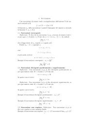
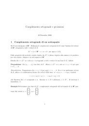
⇒ P 1 = (0, 1), P 2 = (1, 1/2), P 3 = (−1, 1/2), P 4 = ( √ 2, 1), P 5 = (− √ 2, 1)3. Linearizzazione attorno ai punti critici: si considera la matrice jacobiana calcolata nel genericopunto fisso (¯x, ȳ), si ha⎛∂f 1∂x (¯x, ȳ) ∂f⎞1(¯x, ȳ)∂y (A(¯x, ȳ) = ⎜⎟⎝∂f 2∂x (¯x, ȳ) ∂f⎠ = −4(¯x 2 )− 1)¯x 24(ȳ − 1)(3¯x 2 − 1) 4¯x(¯x 2 − 1)2∂y (¯x, ȳ)Scrivo l’equazione secolare e determino gli autovalori della matrice A(ẑ):det[A(¯x, ȳ) − λ1I] = −16¯x 2 (¯x 2 − 1) 2 + λ 2 − 8(ȳ − 1)(3¯x 2 − 1) = 0⇒ λ 1,2 (¯x, ȳ) = ± √ 16¯x 2 (¯x 2 − 1) 2 + 8(ȳ − 1)(3¯x 2 − 1)A questo punto è possibile studiare la stabilità dei punti critici: λ 1,2 (P 1 ) = 0, gli autovalori sono nulli,quindi non si può dire nulla sulla stabilità di P 1 ; λ 1,2 (P 2,3 ) = ±2i √ 2, gli autovalori hanno parte realezero, quindi non si può dire nulla sulla stabilità di P 2 e di P 3 ; λ 1,2 (P 4,5 ) = ±4 √ 2, gli autovalori sono realie distinti; ne esiste uno positivo, quindi P 4 e P 5 sono punti di equilibrio instabile.Metodo di Liapunov: i punti P i , con i = 1, . . . , 5, sono estremali per la funzione u(x, y). Per studiarne leproprietà è necessario scrivere la matrice hessiana H(x, y)e quindiH(x, y) =∂ 2 u∂x 2 = −∂f 2∂x = −4(y − 1)(3x2 − 1)( −4(y − 1)(3x 2 − 1) −4x(x 2 − 1)−4x(x 2 − 1) 2∂ 2 u∂y 2 = ∂f 1∂y = 2)∂ 2 u∂x∂y = ∂2 u∂y∂x = −4x(x2 − 1)e det (H(x, y)) = −8(y−1)(3x 2 −1)−16x 2 (x 2 −1) 2Poiché det (H(P 2,3 )) = 8 > 0 e H 1,1 (P 2,3 ) = 4 > 0 si ha che i punti P 2 e P 3 sono di minimo relativoproprio per la funzione u(x, y). Segue che la funzione w(x, y) := u(x, y) − u(P 2 ) = u(x, y) − u(P 2 ) è unafunzione di Liapunov per P 2 e per P 3 , quindi in virtù del Teorema 2.30 si conclude che i punti fissi P 2 eP 3 sono punti di equilibrio stabile. Sul punto P 1 non si può, invece, dire nulla perché det (H(P 1 )) = 0,ma dallo studio delle curve di livello emergerà che si tratta di un punto di equilibrio instabile.4. Si considerano le curve di livello u(x, y) = a, con a ∈ R. In primo luogo si osserva che u(x, y) è unafunzione pari nella variabile x, quindi le curve di livello avranno l’asse y per asse di simmetria. Inoltreu(P 1 ) = u(P 4 ) = u(P 5 ) = −1, P 4 e P 5 sono punti instabili, le curve di livello più interessanti sono propriole separatrici, cioè quelle passanti per i punti critici instabili. Si studia, ora, la struttura delle curve dilivello al variare del parametro a:– per a = −1, la forma implicita dell’equazione algebrica della curva di livello èy 2 − [ (x 2 − 1) 2 + 1 ] y + x 2 (x 2 − 2) + 1 = 0 ⇒ y 2 − y − (x 2 − 1) 2 y + (x 2 − 1) 2 = 0⇒ y(y − 1) − (y − 1)(x 2 − 1) 2 = 0 ⇒ (y − 1) [ y − (x 2 − 1) 2] = 0quindi la separatrice è costituita dalle due curve di equazione y = 1 e y = (x 2 − 1) 2 , si veda lafigura 2.19. Su tale curva di livello giacciono undici orbite: otto orbite asintotiche ai punti diequilibrio instabili e tre punti di equilibrio instabili.Si osserva che la separatrice divide lo spazio delle fasi in sette regioni connesse; per capire dovesi collocheranno le curve di livello al variare del parametro a è sufficiente calcolare il valore diu in un solo punto di ciascuna di queste regioni e poi usare la continuità della funzione u. Siha u(P 2 ) = u(P 3 ) = −5/2 < −1, u(0, 2) = 0, u(2, 2) = −8 e u(0, 0) = 0. Quindi le curve dilivello giacenti nelle due regioni interne alla separatrice corrispondo a valori di a nell’intervallo−5/2 < a < −1; quelle sovrastanti e sottostanti la separatrice corrispondono ad a > −1; quellenelle due regioni restanti corrispondono ad a < −5/2.fismat05.tex – 20 Aprile 2006 – 13:12 pagina 56
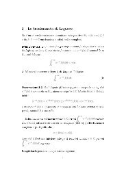
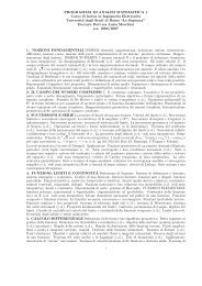
y✻✛− √ 2✲✲ ✲✲✛−1 +1+ √ 2✛✲xFig. 2.19. Curve di livello per il sistema dinamico (2.38). I versi non indicati si deducono per continuità.– Per −5/2 < a < −1, le curve di livello sono costituite da quattro componenti connesse, giacentirispettivamente nelle regioni A 2 := {(x, y) ∈ R 2 : 0 < x < √ 2, (x 2 −1) 2 < y < 1}, A 3 := {(x, y) ∈R 2 : − √ 2 < x < 0, (x 2 − 1) 2 < y < 1}, A 5 := {(x, y) ∈ R 2 : x < − √ 2, 1 < y < (x 2 − 1) 2 } eA 4 := {(x, y) ∈ R 2 : x > + √ 2, 1 < y < (x 2 − 1) 2 }. I due insiemi A 2 e A 3 contengono ciascunoun solo punto di equilibrio stabile, quindi le curve di livello ivi giacenti sono curve chiuse, regolariche ruotano attorno al relativo punto di equilibrio stabile, si veda il Teorema 2.22. Su ciascunacomponente connessa di ogni curva di livello giace un’orbita, le orbite con dato iniziale nelle regioniA 2 e A 3 sono periodiche attorno al relativo punto di equilibrio stabile, si veda la figura 2.19.– Per a > −1 le curve di livello u(x, y) = a sono quelle disegnate per continuità in figura e giavccionorispettivamente in A 1,− := {(x, y) ∈ R 2 : x < − √ 2 e y < 1, − √ 2 < x < √ 2 e y < (x 2 − 1) 2 , x >+ √ 2 e y < 1} e A 1,+ := {(x, y) ∈ R 2 : x < − √ 2 e y > (x 2 − 1) 2 , − √ 2 < x < √ 2 e y > 1, x >+ √ 2 e y > (x 2 − 1) 2 }. Ogni curva è costituita da due componenti connesse aperte su ciascunadelle quali giace una sola linea di fase.– Per a < −5/2 le curve di livello u(x, y) = a sono quelle disegnate per continuità in figura egiacciono rispettivamente in A 4 e A 5 . Ogni curva è costituita da due componenti connesse apertesu ciascuna delle quali giace una sola linea di fase.I versi sulla separatrice vengono determinati ricordando che su un tratto di curva di livello che noninterseca alcun punto di equilibrio il verso non cambia e osservando che f 1 (1, 1) = 1 > 0, f 1 (1, 0) = −1 0. Sulle altre curve di livello i versi possono essere trovati percontinuità. Dalla discussione precedente si ha che l’insieme dei dati iniziali che generano orbite periodicheè Π = D 2 ∪ D 3 .5. Si consideri l’orbita generata dal dato iniziale (x 0 , y 0 ) = (1, 3/4). Poiché (x 0 , y 0 ) ∈ D 2 si ha chel’orbita uscente è periodica. Per poter scrivere il periodo dell’orbita è necessario scrivere l’equazionedella curva di livello in forma esplicita, cioè si deve ricavare y in funzione di x o viceversa; ponendou(x, y) = u(x 0 , y 0 ) si trovay 2 − [ (x 2 − 1) 2 + 1 ] y + x 2 (x 2 − 1) = − 1916 ⇒ y2 − [ (x 2 − 1) 2 + 1 ] y + x 2 (x 2 − 1) + 1 = − 3 16 ⇒(y − 1) [ y − (x 2 − 1) 2] = − 3 16 ⇒ (x2 − 1) 2 = y +316(y − 1)Dalla precedente si può ricavare la variabile x in funzione della variabile y semplicemente eseguendo delleradici quadrate. Bisogna, però controllare che i radicandi siano positivi: il secondo membro è positivo see solo se 16y 2 − 16y + 3 ≤ 0, ovvero se 1/4 ≤ y ≤ 3/4. Da questa osservazione si deduce che l’orbita ècompresa tra le due rette y = 1/4 e y = 3/4 e le tocca nei punti (x 0 , y 0 ) = (1, 3/4) e (x 1 , y 1 ) = (1, 1/4).Quindi per i valori di y permessi si ha:x 2 − 1 = ±√y +316(y − 1)fismat05.tex – 20 Aprile 2006 – 13:12 pagina 57
Page 1 and 2:
Esercizi e appunti per il corso di
Page 3 and 4:
⇒ x(t) = Ce tcon C ∈ RImpondend
Page 5 and 6: ✻x✟✻✟ ✟ ✟ ✟x✻x 0x
Page 7 and 8: viene scelto vicino a x 2 il sistem
Page 9 and 10: Esercizio 1.4. Supponendo uniforme
Page 11 and 12: Questo è parzialmente vero nel cas
Page 13 and 14: L’integrale, infatti, ha senso pe
Page 15 and 16: sensato, perché si ricorda che le
Page 17 and 18: dimostrare che il tempo t 1 − t 0
Page 19 and 20: con f : R n → R una funzione asse
Page 21 and 22: Come nel caso unidimensionale verif
Page 23 and 24: - asintoticamente stabile se e solo
Page 25 and 26: Esempio 2.9. Sulla base di argoment
Page 27 and 28: x 2✻✲✻ ✲✛ ✻❄✛ ❄
Page 29 and 30: Per esempio nel punto ¯x = (0, 1)
Page 31 and 32: livello chiusa, questa osservazione
Page 33 and 34: (x 2 + y 2 )/2. Si può verificare
Page 35 and 36: - Per a = 1, la curva di livello pa
Page 37 and 38: Teorema 2.21 Si consideri il sistem
Page 39 and 40: ciò fa intuire che in qualche sens
Page 41 and 42: Teorema 2.28 (Stabilità dei sistem
Page 43 and 44: La palla B δ (x e ) è proprio que
Page 45 and 46: e si studia la matrice associata al
Page 47 and 48: −ω 2 sin θ, dove ω = √ g/l
Page 49 and 50: Da questa proprietà segue che w è
Page 51 and 52: ✲✲✛✛P 3p✻✲✲✛✛P 2
Page 53 and 54: −πp✲✻✲✲ ✲✛0 π q✛
Page 55: è soddisfatta, perché L f ′w(q,
Page 59 and 60: Esercizio 2.16. Per i seguenti sist
Page 61 and 62: degli assi cartesiani dello spazio
Page 63 and 64: Dal momento che I 1 < I 2 < I 3 si
Page 65 and 66: Il problema (3.1) può essere ricon
Page 67 and 68: dell’analisi avendo come riferime
Page 69 and 70: Γ e = {(q, p) ∈ R 2 : q e 1 ≤
Page 71 and 72: Osservato che dall’equazione dell
Page 73 and 74: assunto nel minimo, cioè a zero. I
Page 75 and 76: La tesi, allora, segue in virtù de
Page 77 and 78: u(q)✻q 3 q 4 q 1 q 2✲ qu 0p
Page 79 and 80: p✻q0(q − q 0 ) 1/2 p (q − q 0
Page 81 and 82: Si può osservare che ˙θ ha segno
Page 83 and 84: Troncando lo sviluppo delle potenze
Page 85 and 86: deve specificare il valore della ca
Page 87 and 88: valore della soluzione sull’asse
Page 89 and 90: x ∈ [a, b], u x (a, t) = u 1,a (t
Page 91 and 92: Inoltre si è usata l’identità n
Page 93 and 94: con q = (x, y, z) ∈ R 3 , t ∈ R
Page 95 and 96: Le equazioni del moto possono esser
Page 97 and 98: Sostituendo queste espressioni nell
Page 99 and 100: 1. u x + u y = u;2. 2u x − 3u y =
Page 101 and 102: In realtà lo studio è limitato al
Page 103 and 104: 3. u(x, y) = log √ x 2 + y 2 , (x
Page 105 and 106: nella regione√2E := {(ξ, η) ∈
Page 107 and 108:
ammette l’unica soluzioneu(x, t)
Page 109 and 110:
Esercizio 6.43. Una corda semi-illi
Page 111 and 112:
Esercizio 6.50. Come l’Esercizio
Page 113 and 114:
Esercizio 6.59. Per effetto di una
Page 115 and 116:
Esercizio 6.66. Si risolva l’equa
Page 117 and 118:
4. u 0 (x) = exp{−α|x|} con α
Page 119:
6.3. Equazione di Laplace: funzioni
show all

Esercizi e appunti per il corso di Fisica Matematica - Sezione di ...

You also want an ePaper? Increase the reach of your titles

Delete template?

Save as template?