Modelos para Dados de Contagem com Estrutura Temporal
Modelos para Dados de Contagem com Estrutura Temporal
Modelos para Dados de Contagem com Estrutura Temporal

You also want an ePaper? Increase the reach of your titles
YUMPU automatically turns print PDFs into web optimized ePapers that Google loves.
<strong>com</strong> Ỹt =<br />
Ỹt(θ<br />
(j−1)<br />
t<br />
) e V t = V t (θ (j−1)<br />
t ), em que θ (j−1)<br />
t<br />
θ T , a distribuição proposta é uma distribuição normal <strong>com</strong> variância<br />
e média<br />
<strong>com</strong> ỸT = ỸT (θ (j−1)<br />
T<br />
é o valor corrente da ca<strong>de</strong>ia. Para<br />
B T = (F T V −1<br />
T<br />
F′ T + W −1<br />
T )−1 (2.25)<br />
b T = B T (F T V −1<br />
T<br />
Ỹ T + W −1<br />
T G T θ T −1 ), (2.26)<br />
) e V T = V T (θ (j−1)<br />
T<br />
), em que θ (j−1)<br />
T<br />
é o valor corrente da ca<strong>de</strong>ia.<br />
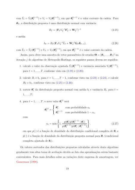
Assim, <strong>para</strong> obter uma amostra do vetor <strong>para</strong>métrico <strong>de</strong> estados Θ = (θ 1 , . . . , θ T ) ′ na<br />
iteração j do algoritmo <strong>de</strong> Metropolis-Hastings, os seguintes passos <strong>de</strong>vem ser seguidos:<br />
1. calcule o valor da observação ajustada<br />
<strong>para</strong> t = 1, . . . , T , conforme visto em (2.19) e (2.20);<br />
(j−1) Ỹt(θ t ) e variância associada V t (θ (j−1)<br />
t ),<br />
2. calcule B t e b t , <strong>para</strong> t = 1, . . . , T − 1, conforme visto em (2.23) e (2.24), e calcule<br />
B T e b T , conforme visto em (2.25) e (2.26);<br />
3. sorteie θ ∗ t da distribuição proposta normal <strong>com</strong> média b t e variância B t , <strong>para</strong> t =<br />
1, . . . , T ;<br />
4. <strong>para</strong> t = 1, . . . , T , o novo valor θ (j)<br />
t será<br />
⎧<br />
⎨<br />
<strong>com</strong><br />
θ (j)<br />
t =<br />
⎩<br />
θ ∗ t<br />
<strong>com</strong> probabilida<strong>de</strong> α t<br />
θ (j−1)<br />
t <strong>com</strong> probabilida<strong>de</strong> 1 − α t ,<br />
{<br />
}<br />
p(θ ∗ t )˜p(θ (j−1)<br />
t | θ ∗ t )<br />
α t = min 1,<br />
, (2.27)<br />
p(θ (j−1)<br />
t )˜p(θ ∗ t | θ (j−1)<br />
t )<br />
em que p(·) é a função <strong>de</strong> <strong>de</strong>nsida<strong>de</strong> da distribuição condicional <strong>com</strong>pleta <strong>de</strong> θ t e<br />
˜p(·) é a função <strong>de</strong> <strong>de</strong>nsida<strong>de</strong> da distribuição proposta normal <strong>para</strong> θ t (condicional<br />
<strong>com</strong>pleta ajustada <strong>de</strong> θ t ).<br />
Os valores sorteados das distribuições propostas calculadas através <strong>de</strong>sta algoritmo<br />
geralmente tem altas taxas <strong>de</strong> aceitação <strong>de</strong>vido ao fato das aproximações serem bastante<br />
convenientes. Para mais <strong>de</strong>talhes sobre as variações <strong>de</strong>ste esquema <strong>de</strong> amostragem, ver<br />
Gamerman (1998).<br />
19