Modelagem Física e Computacional de um Escoamento Fluvial

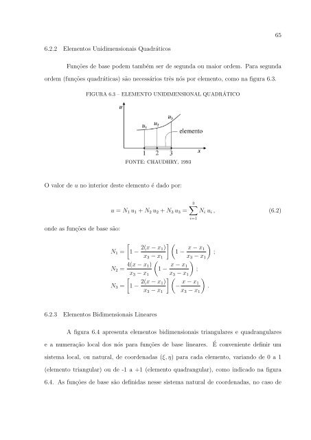
6.2.2 Elementos Unidimensionais Quadráticos
Funções de base podem também ser de segunda ou maior ordem. Para segunda
ordem (funções quadráticas) são necessários três nós por elemento, como na figura 6.3.
FIGURA 6.3 – ELEMENTO UNIDIMENSIONAL QUADR ÁTICO
FONTE: CHAUDHRY, 1993
O valor de u no interior deste elemento é dado por:
onde as funções de base são:
u = N1 u1 + N2 u2 + N3 u3 =
65
3
Ni ui , (6.2)
i=1
2(x − x1) x − x1
N1 = 1 − 1 − ;
x3 − x1 x3 − x1
4(x − x1) x − x1
N2 = 1 − ;
x3 − x1 x3 − x1
2(x − x1) x − x1
N3 = 1 − − .
x3 − x1
6.2.3 Elementos Bidimensionais Lineares
x3 − x1
A figura 6.4 apresenta elementos bidimensionais triangulares e quadrangulares
e a numeração local dos nós para funções de base lineares.
É conveniente definir um
sistema local, ou natural, de coordenadas (ξ, η) para cada elemento, variando de 0 a 1
(elemento triangular) ou de -1 a +1 (elemento quadrangular), como indicado na figura
6.4. As funções de base são definidas nesse sistema natural de coordenadas, no caso de