Identification des mécanismes de fissuration dans un alliage d ...
Identification des mécanismes de fissuration dans un alliage d ...
Identification des mécanismes de fissuration dans un alliage d ...

Create successful ePaper yourself
Turn your PDF publications into a flip-book with our unique Google optimized e-Paper software.
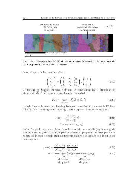
124 Etu<strong>de</strong> <strong>de</strong> la <strong>fissuration</strong> sous chargement <strong>de</strong> fretting et <strong>de</strong> fatigue<br />
contraste <strong>de</strong> ban<strong><strong>de</strong>s</strong><br />
très faible près<br />
<strong>de</strong> la fissure<br />
on extrait la<br />
matrice d’orientation<br />
<strong>de</strong> chaque grain<br />
X ‖ L<br />
Y ‖ T<br />
Fig. 3.51: Cartographie EBSD d’<strong>un</strong>e zone fissurée (essai 3), le contraste <strong>de</strong><br />
ban<strong><strong>de</strong>s</strong> permet <strong>de</strong> localiser la fissure.<br />
<strong>dans</strong> le repère <strong>de</strong> l’échantillon alors :<br />
⎛<br />
⎝<br />
⎞ ⎛<br />
n x<br />
n y<br />
⎠ = ⎝<br />
n z<br />
⎞<br />
b 11 b 12 b 13<br />
b 21 b 22 b 23<br />
⎠ .<br />
b 31 b 32 b 33<br />
⎛<br />
⎝<br />
⎞<br />
n 1<br />
n 2<br />
⎠ (3.19)<br />
n 3<br />
Le facteur <strong>de</strong> Schmid du plan s’obtient en considérant les 3 directions <strong>de</strong><br />
glissement ( ⃗ d 1 , ⃗ d 2 , ⃗ d 3 ) associées au plan et en calculant :<br />
FS j = max<br />
i=1,2,3<br />
| ⃗ N j . ⃗ X × ⃗ d i . ⃗ X| (3.20)<br />
L’angle θ entre la trace du plan <strong>de</strong> glissement considéré à la surface <strong>de</strong> l’échantillon<br />
et l’axe <strong>de</strong> chargement (voir fig. 3.50) s’exprime <strong>dans</strong> notre cas par :<br />
cos(θ) = ( ⃗ N ∧ ⃗ Z)<br />
|| ⃗ N ∧ ⃗ Z|| . ⃗ X<br />
θ = arctan(−n x /n y )<br />
(3.21)<br />
(3.22)<br />
Enfin, l’angle <strong>de</strong> twist entre <strong>de</strong>ux plans <strong>de</strong> <strong>fissuration</strong>s successifs (N 1 <strong>dans</strong> le grain<br />
1 et N 2 <strong>dans</strong> le grain 2 par exemple) se calcule en projetant les <strong>de</strong>ux plans mis<br />
en jeu sur le joint <strong>de</strong> grain supposé perpendiculaire à la surface et à la direction<br />
<strong>de</strong> chargement :<br />
cos(α) = ( N ⃗ 2 ∧ X) ⃗<br />
|| N ⃗ 2 ∧ X|| ⃗ . ( N ⃗ 1 ∧ X) ⃗<br />
|| N ⃗ 1 ∧ X|| ⃗<br />
α = | arctan(−n 2 z/n 2 y) − arctan(−n 1 z/n 1 y) |<br />
} {{ } } {{ }<br />
déflection déflection<br />
du plan 2 du plan 1<br />
(3.23)<br />
(3.24)