Identification des mécanismes de fissuration dans un alliage d ...

3.4 Propagation de fissures amorcées en fretting sous chargement de fatigue 135
3.4.1 Observations quantitatives sur la propagation
Devant la richesse des informations recueillies par tomographie, un seul essai in
situ est détaillé dans cette partie. L’analyse de la fissure de fretting a été présentée
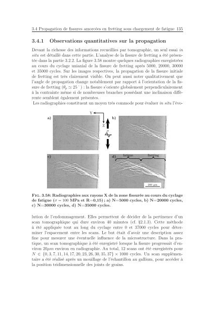
dans la partie 3.2.2. La figure 3.58 montre quelques radiographies enregistrées
au cours du cyclage uniaxial de la fissure de fretting après 5000, 20000, 30000
et 35000 cycles. Sur les images respectives, la propagation de la fissure initiale
de fretting est très clairement visible. On peut aussi noter qualitativement que
l’angle de propagation change notablement par rapport à l’orientation de la fissure
de fretting (θ p ≃ 25˚) : la fissure s’oriente globalement perpendiculairement
à la contrainte même si de nombreuses branches possédant une inclinaison différente
semblent également présentes.
Les radiographies constituent un moyen très commode pour évaluer in situ l’évo-
Y
a) b)
Z
σ
c) d) fatigue fretting
200 µm
Fig. 3.58: Radiographies aux rayons X de la zone fissurée au cours du cyclage
de fatigue (σ = 100 MPa et R=0,15); a) N=5000 cycles, b) N=20000 cycles,
c) N=30000 cycles, d) N=35000 cycles.
lution de l’endommagement. Elles permettent de décider de la pertinence d’un
scan tomographique qui dure environ 40 minutes (cf. §2.1.3). Cette méthode
à été appliquée tout au long du cyclage entre 0 et 37000 cycles pour déterminer
l’espacement entre les scans. Le but était d’avoir une description assez
fine pour mesurer une éventuelle influence de la microstructure. Dans la pratique,
un scan tomographique à été enregistré lorsque la fissure progressait d’environ
20µm environ en radiographie. Au total, 12 scans ont été enregistrés pour
N ∈ {0, 3, 7, 11, 14, 17, 20, 23, 26, 30, 35, 37} × 1000 cycles. Un scan supplémentaire
a été réalisé après un mouillage de l’échantillon au gallium, pour accéder à
la position tridimensionnelle des joints de grains.