Campos de Vetores Polinomiais Planares: Análise ... - Unesp

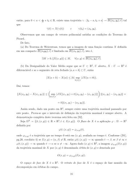
então, para 0 < a < r M
que
e t 0 ∈ R, existe uma trajetória γ : [t 0 − a, t 0 + a] → B((x 0 , y 0 ), r) tal
˙γ(t) = X(γ(t)) e γ(t 0 ) = (x 0 , y 0 ).
Observemos que um campo de vetores polinomial satisfaz as condições do Teorema de
Picard.
De fato,
(a) Do Teorema de Weierstrass, temos que a imagem de uma função contínua X definida
em um compacto B((x 0 y 0 ), r) é limitada em B((x 0 , y 0 ), r), isto é,
∃M > 0, ‖X(x, y)‖ ≤ M,
∀(x, y) ∈ B((x 0 , y 0 ), r).
(b) Da Desigualdade do Valor Médio segue que se U ⊂ R 2 , U aberto, X : U → R 2 é
diferenciável e se o segmento de reta fechado [a, a + h] ⊂ U, então
Daí, temos:
|X(a + h) − X(a)| ≤ |h| sup |JX(a + th)|.
0≤t≤1
(
)
‖X(x 2 , y 2 ) − X(x 1 , y 1 )‖ ≤ sup |JX[(x 1 , y 1 ) + t((x 2 , y 2 ) − (x 1 , y 1 ))]|
0≤t≤1
‖(x 1 , y 1 ) − (x 2 , y 2 )‖ =
= k‖(x 1 , y 1 ) − (x 2 , y 2 )‖.
Assim sendo, dado um ponto em R 2 , sempre existe uma trajetória maximal passando por
este ponto. Prova-se que o intervalo de definição da trajetória maximal é sempre aberto. A
demonstração completa deste teorema está feita em [S2].
Seja Ω X = {(t, (x, y)) ∈ R × R 2 , t ∈ I(x, y)}. O fluxo de X é a aplicação ϕ : Ω → R 2
definida por
ϕ(t, (x, y)) = ϕ (x,y) (t),
onde ϕ (x,y) é a trajetória que no tempo 0 está em (x, y), avaliada no tempo t. Conforme ([S1],
pg.20, corolário 4) se I(x, y) = (α, β) ≠ R, então ϕ(t, (x, y)) → ∞ quando t → β, se β ≠ ∞ e
ϕ(t, (x, y)) → ∞ quando t → α se α ≠ −∞. Agora dado (x, y) ∈ R 2 , a imagem ϕ (x,y) (I(x, y))
da trajetória maximal de X por (x, y) é denominada órbita de (x, y) e denotada por
O(x, y) = ϕ (x,y) (I(x, y)).
O espaço de fase de X é o R 2 .
decomposição em órbitas do campo.
O retrato de fase de X é o espaço de fase munido da
16