Campos de Vetores Polinomiais Planares: Análise ... - Unesp
Campos de Vetores Polinomiais Planares: Análise ... - Unesp
Campos de Vetores Polinomiais Planares: Análise ... - Unesp

You also want an ePaper? Increase the reach of your titles
YUMPU automatically turns print PDFs into web optimized ePapers that Google loves.
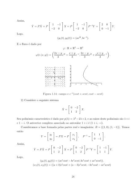
Assim,<br />
Ẏ = P Ẋ = P [<br />
1 −1<br />
−2 0<br />
] [<br />
X = P<br />
1 −1<br />
−2 0<br />
] [<br />
P −1 Y =<br />
2 0<br />
0 −1<br />
]<br />
Y.<br />
Logo,<br />
(y 1 (t), y 2 (t)) = (ae 2t , be −t ).<br />
E o fluxo é dado por<br />
( 2x − y<br />
ϕ(t, (x, y)) =<br />
3<br />
ϕ : R × R 2 → R 2<br />
e 2t + x + y<br />
3<br />
e −t , 2x − y<br />
3<br />
e 2t + 2 x + y )<br />
e −t .<br />
3<br />
Figura 1.14: campo e e −t (cost + sent, cost − sent)<br />
2) Consi<strong>de</strong>re o seguinte sistema<br />
Ẋ =<br />
[<br />
0 −2<br />
1 2<br />
]<br />
X.<br />
Seu polinômio característico é dado por p(λ) = λ 2 − 2λ + 2, e as raízes <strong>de</strong>ste polinômio são 1 + i<br />
e 1 − i. O autovetor complexo associado ao autovalor 1 + i é (1 + i, −i).<br />
então<br />
Assim,<br />
Logo,<br />
Consi<strong>de</strong>ramos a base formada pelas partes real e imaginária: B = {(1, 0), (1, −1)}. Temos<br />
Y =<br />
[<br />
Ẏ = P Ẋ = P [<br />
]<br />
[<br />
y 1<br />
= P X = P<br />
y 2<br />
0 −2<br />
1 2<br />
]<br />
X = P<br />
] [<br />
x 1<br />
, P −1 =<br />
x 2<br />
[<br />
0 −2<br />
1 2<br />
]<br />
P −1 Y =<br />
1 1<br />
0 −1<br />
[<br />
]<br />
.<br />
1 −1<br />
1 1<br />
(y 1 (t), y 2 (t)) = (ae t cost − be t sent, be t cost + ae t sent)).<br />
(x 1 (t), x 2 (t)) = ((a + b)e t cost + (a − b)e t sent, −be t cost − ae t sent)<br />
]<br />
Y.<br />
26