Campos de Vetores Polinomiais Planares: AnÃ¡lise ... - Unesp

More documents

Recommendations

Info

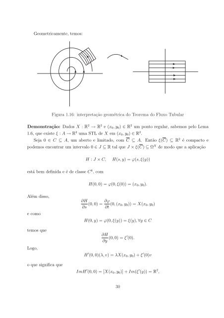
Geometricamente, temos: Figura 1.16: interpretação geométrica do Teorema do Fluxo Tubular Demonstração: Dados X : R 2 → R 2 e (x 0 , y 0 ) ∈ R 2 um ponto regular, sabemos pelo Lema 1.6, que existe ξ : A → R 2 uma STL de X em (x 0 , y 0 ) ∈ R 2 . Seja 0 ∈ C ⊆ A, um aberto e limitado, com C ⊆ A. Então ξ(C) ⊆ R 2 é compacto e podemos encontrar um intervalo 0 ∈ J ⊆ R tal que J × ξ(C) ⊆ Ω X de modo que a aplicação H : J × C, H(s, y) = ϕ(s, ξ(y)) está bem definida e é de classe C k , com H(0, 0) = ϕ(0, ξ(0)) = (x 0 , y 0 ). Além disso, e como temos que Logo, o que significa que ∂H ∂ϕ (0, 0) = ∂s ∂t (0, (x 0, y 0 )) = X(x 0 , y 0 ) H(0, y) = ϕ(0, ξ(y)) = ξ(y), ∀y ∈ C ∂H ∂y (0, 0) = ξ′ (0). H ′ (0, 0)(λ, v) = λX(x 0 , y 0 ) + ξ ′ (0)v ImH ′ (0, 0) = [X(x 0 , y 0 )] + Im(ξ ′ (y)) = R 2 , 30
ou seja, H ′ (0, 0) : R × R → R 2 é uma transformação linear sobrejetiva, e portanto um isomorfismo. Do Teorema da Aplicação Inversa decorre que H é um difeomorfismo de classe C ∞ em (0, 0), isto é, existem um intervalo I = (−δ, δ) ⊆ J ⊂ R, uma vizinhança 0 ∈ B ⊆ C ⊆ A ⊂ R e uma vizinhança W 0 de (x 0 , y 0 ) em R 2 tal que h : I × B → W 0 definida pela restrição h(s, y) = H(s, y) é um difeomorfismo de classe C k . Daí, temos que: h(0, 0) = (x 0 , y 0 ), h(0, y) = ξ(y), h({0} × B) = ξ(B). Agora como temos que h conjuga X e Y . h ′ (s, y)Y (s, y) = H ′ (s, y)(1, 0) = ∂H ∂s ∂ϕ (s, y) = (0, ξ(y)) = ∂t = X(ϕ(s, ξ(y))) = X(h(s, y)), ∀(s, y) ∈ I × B 1.4 Estrutura Local dos Pontos Singulares Hiperbólicos: Teorema de Grobman-Hartman Pelo Teorema do Fluxo Tubular, sabemos que existe um difeomorfismo (de classe C r ) que conjuga X em uma vizinhança de um ponto regular (x 0 , y 0 ) com o campo constante Y = (1, 0). Daí, dois campos X e Y são localmente conjugados em torno de pontos regulares. Por esse motivo, temos um conhecimento satisfatório das órbitas de um campo vetorial polinomial planar em torno dos pontos regulares, visto que existe apenas uma classe de conjugação diferencial local. Se (x 0 , y 0 ) é uma singularidade, a situação é bem mais complicada. Vamos então analisar nesta seção as singularidades hiperbólicos, isto é, os pontos onde todos os autovalores da JX(x 0 , y 0 ) tem parte real diferente de 0 e também o Teorema de Grobman-Hartman: Teorema 1.8 (Grobman-Hartman). Seja X : R 2 → R 2 um campo vetorial polinomial e (x 0 , y 0 ) um ponto singular hiperbólico. Então existem V ⊂ R 2 , com (x 0 , y 0 ) ∈ V e W ∈ R 2 , com (0, 0) ∈ W tal que X/V é topologicamente equivalente a JX(x 0 , y 0 )/W . 31
Page 1: Campos de Vetores Polinomiais Plana
Page 5: Agradecimentos Ao Prof. Dr. Paulo R
Page 9: Abstract In this work we present ba
Page 12 and 13: Referências Bibliográficas 115 12
Page 14 and 15: mas logo nos convencemos da complex
Page 16 and 17: então, para 0 < a < r M que e t 0
Page 18 and 19: 1.2 Primeiros Exemplos: Campos de V
Page 20 and 21: Figura 1.4: α = β < 0, α < β <
Page 22 and 23: (ii) Se [A] B = [ λ 1 0 λ ] , ent
Page 24 and 25: Se β < 0 o campo de vetores é do
Page 26 and 27: Assim, Ẏ = P Ẋ = P [ 1 −1 −
Page 28 and 29: onde p e q são polinômios de grau
Page 32 and 33: Geometricamente, temos: ( 0 x 0 , y
Page 34 and 35: para todo t ≥ 0. Ainda ϕ(t, (x,
Page 36 and 37: 1.6 Conjuntos α-limites e ω-limit
Page 38 and 39: Como τ é contínua, temos que lim
Page 40 and 41: Suponha que o campo X possua um nú
Page 42 and 43: e E U = [{u j , v j }/a j > 0] isto
Page 44 and 45: Portanto, temos que x(t) = e λ 1t
Page 46 and 47: Temos que o primeiro valor é dado
Page 48 and 49: espectivamente. Pode ser mostrado q
Page 50 and 51: Definição 2.5. Uma singularidade
Page 52 and 53: e ˙θ = 1. Assim, r(t) = r 0 (1−
Page 54 and 55: (0,0) Figura 2.8: sela topológica
Page 56 and 57: isto é, θ = tg −1 ( 3 ± √ )
Page 58 and 59: por zero; além disso, o seguinte l
Page 60 and 61: tem uma determinada vizinhança con
Page 62 and 63: onde p 2 e q 2 são polinômios e t
Page 64 and 65: Exemplo 2.28. Considere o sistema {
Page 66 and 67: C W (0) S S E = W (0) E C Figura 2.
Page 68 and 69: Quando {y ≠ 0}, (3.2) também ser
Page 70 and 71: Para θ = 0, 5880, temos: [ JX(0; 0
Page 72 and 73: Logo, temos { ˙¯x = −¯x 2 −
Page 74 and 75: 3.0.1 Blow-up Quase-homogêneo e o
Page 76 and 77: com ¯x 2 + ȳ 2 = 1. Vamos testar
Page 78 and 79: Calculando a sua matriz jacobiana,
Page 80 and 81:
Consideremos o problema de Cauchy {
Page 82 and 83:
Como x = rCsθ e y = r 2 Snθ, temo
Page 84 and 85:
Passando este sistema de equações
Page 86 and 87:
E o seu retrato de fase é dado pel
Page 88 and 89:
elementares, introduzimos ŷ = ȳ
Page 90 and 91:
Capítulo 4 Compactificação de Po
Page 92 and 93:
Z y (x,y) x (X,Y,Z) Y X (X`,Y`,Z`)
Page 94 and 95:
A equação diferencial (4.5) defin
Page 96 and 97:
Figura 4.5: Projeção de S 2 nos p
Page 98 and 99:
Disto concluímos que os pontos cr
Page 100 and 101:
Capítulo 5 O Programa P4 O program
Page 102 and 103:
utilizando a invariância do fluxo,
Page 104 and 105:
senão S = [L p 1, ..., L n N p , L
Page 106 and 107:
- L p N p = [[T 1 , ..., T l , (x,
Page 108 and 109:
forma a ser o máximo de δ. Com um
Page 110 and 111:
um ponto da Esfera de Poincaré com
Page 112 and 113:
o P4 primeiro considera o campo de
Page 114 and 115:
um ciclo limite na circunferência
Page 116:
[Ne] Neumann, D. Classification of
show all

Campos de Vetores Polinomiais Planares: AnÃ¡lise ... - Unesp

Create successful ePaper yourself

Delete template?

Save as template?