Download - Academy Publisher

model that can deal with time series data based on the
Probability Network. It considers factors outside the
system as well as the inter-link
A DBN consist of two parts (a priori Network and
Transition Network), having which a DBN will be formed
in any length. To facilitate the processing, we suppose the
DBN can meet the conditions: (a).the network topology
dose not change over time; (b) the network meet the
first-order Markov condition. Satisfying the above two
conditions the DBN can be seen as unfolding in time
sequence.
Compared with the existing works, we use a stronger
temporal signal processor-----DBN (Dynamic Bayesian
Network) [16] to identify the shot event. On the one hand,
considering the transition probability between the various
moments, dynamic Bayesian networks extend Bayesian
network modeling capabilities of the timing signals. On
the other hand, dynamic Bayesian networks allow the use
of multiple state variables at the same point in time, while
Hidden Markov model uses only one state variable. Based
on these considerations, we believe that Dynamic
Bayesian Networks is more suitable for sports video
content analysis, especially for the semantic analysis of
events and their mutual relations.
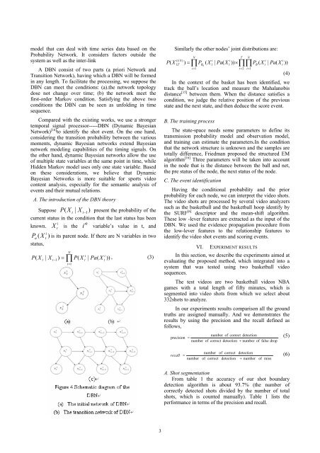
A. The introduction of the DBN theory
Suppose P ( X t
| X t− 1)
present the probability of the
current status in the condition that the last status has been
i
known. X
t
is the i th variable’s value in t, and
i
Pa ( X t
) is its parent node. If there are N variables in two
status,
t
N
t− ) = ∏
i=
1
P( X | X
1
P(
X | Pa(
X )) , (3)
i
t
i
t
Similarly the other nodes’ joint distributions are:
N
T N
(1: N)
i
i
i
i
( X1 : T
) = ∏PB
( X1
| Pa(
X1
)) × ∏∏PB
( X
t
| Pa(
X
t
))
0
i= 1 t= 2 i=
1
P
In the context of the basket has been identified, we
track the ball’s location and measure the Mahalanobis
distance [15] between them. When the distance satisfies a
condition, we judge the relative position of the previous
state and the next state, and then deduce the score event.
B. The training process
The state-space needs some parameters to define its
transmission probability model and observation model,
and training can estimate the parameters.In the condition
that the network structure is unknown and the samples are
totally difference, Friedman proposed the structured EM
algorithm [16] Three parameters will be taken into account
in the node that is the distance between the ball and net,
the pre status of the node, the next status of the node.
C. The event identification
Having the conditional probability and the prior
probability for each node, we can interpret the video shots.
The video shots are processed by several video analyzers
such as the basketball and the basketball hoop identify by
the SURF [6] descriptor and the mean-shift algorithm.
These low -lever features are extracted as the input of the
DBN. We used the evidence propagation procedure from
the low-lever features to the relationship features to
identify the video shot events and scoring events.
VI. EXPERIMENT RESULTS
In this section, we describe the experiments aimed at
evaluating the proposed method, which integrated into a
system that was tested using two basketball video
sequences.
The test videos are two basketball videos NBA
games with a total length of fifty minutes, which is
segmented into video shots from which we select about
332shots to analyze.
In our experiments results comparison all the ground
truths are assigned manually. And we demonstrates the
results by using the precision and the recall defined as
follows,
number of correct detection (5)
precision =
number of correct detection + number
of false drop
(4)
recall =
number
number of correct
of correct detection
detection
+ number
of
miss
(6)
A. Shot segmentation
From table 1 the accuracy of our shot boundary
detection algorithm is about 93.7% (the number of
correctly detected shots divided by the number of total
shots, which is counted manually). Table 1 lists the
performance in terms of the precision and recall.
3