Download - Academy Publisher

A second-order centered difference scheme is applied
to approximate the time derivatives, and a fourth-order
staggered scheme with centered differences to
approximate the spatial derivatives. From Eqs.1, for
n
σ + xy
examples, ,
n
r +
xy
and
n 1
v +
x
can be approximated as:
+ + p + + n +
n +
+ −
( , ) ( , ) ( , ) vy
(, i j )
n + + n + + τ ⋅π
i j τε
i j ∂vx
i j ∂
σ
xy
( i , j ) = σxy
( i , j ) + ( + )
+ +
τσ
( i , j ) ∂y
∂x
(5)
τ
+
n−
n
+ ( rxy
( i, j) + rxy
( i, j))
2
+
n + + τ −1
τ
n − + +
rxy
( i , j ) = (1 + ) ((1 − ) ⋅rxy
( i , j ) −
+ + + +
2 τσ
( i , j ) 2 τ ( i , j )
(6)
σ
+ + s + + n +
n +
τ ⋅ μ( i , j ) τ ( i , j ) v ( , ) vy
(, i j )
(
ε
∂ 1) (
x
i j ∂
− ⋅ +
+ + + +
))
τσ
( i , j ) τσ
( i , j ) ∂y
∂x
+
n
( , )
1 (, )
( , ) ( , ) ( i + j +
+
n
n n τ ∂σ
xy σ i j
+
+ + +
∂
xx
n
vx i j = vx i j + + + fx
) (7)
+
ρ( i , j)
∂y
∂x
Where i, j, k, n are the indices for the three spatial
directions and time, respectively.τ denotes the size of a
timestep.
The discretion of the spatial differential operator, for
example,is given:
+
∂vi
( , j) 1
= (1(( c ⋅ v i+ 1, j ) − v (, i j )) + c 2(( ⋅ v i+ 2, j ) −v ( i−
1, j ))) (8)
∂x
l
Where l denotes grid spacing and c1, c2 denote the
differential coefficients.
B. PML absorbing boundary condition
In order to simulate an unbounded medium, an
absorbing boundary condition (ABC) must be
implemented to truncate the computational domain in
numerical algorithms. Since the highly effective
perfectly matched layer (PML) method [13] for
electromagnetic waves was proposed, the PML has been
widely used for finite-difference and finite-element
methods [14]. The effectiveness of the PML for elastic
waves in solids and the zero reflections from PML to the
regular elastic medium were proved [15].
III. IMPLEMENTATION ON GPUS
A. Overview
To compute the staggered-grid FD and PML equations
on graphics hardware, we divide the geophysical model
into regions represented as textures with the input and
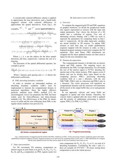
output parameters. Fig.1 shows the division of a 2D
model into a collection of regions. Two sets of
alternating textures binding with a FBO are used to
represent the parameters for computing frame at time t
and t+1 respectively. All the other input-only variables
are stored similarly in 2D textures. To update FBO
textures at each time step, we render quadrilaterals
(regions) mapped with the textures in order, so that a
fragment program running at each texel computes the FD
equations. After each frame, FBO attachments are
swapped and the latest updated textures are then used as
inputs for the next simulation step.
B. Domain decomposition
The computational domain is divided into an interior
region and PML regions. The outgoing waves are
absorbed by the PML via high attenuation. For 2D model,
the size of the interior region is N1*N2, denoting the
interior part of the whole textures. PML region covers 8
blocks and can be divides three types based on the
computing process: PML1, processing absorbing
condition both in x and z direction, with the size
NBC*NBC; PML2 only in z direction and PML3 only in
x direction. The vertex processors will transform on
computational domains and the rasterizer will determine
all the pixels in the output buffer they cover and generate
fragments.
In our approach, velocity and stress fields are
staggered in spatial and time domain. Therefore, the
velocity field is updated after the stress field is updated
and the priority of subdomains processing is interior
region, PML2 (3), PML3 (2), PML1.
0
PML_1
X
PML_2
PML_1
NBC
Frame t+1
N=1-N
Swap
Frame t
Z
PML_3
PML_1
Interior Region
N2=Height-2*NBC PML_3
N1=Width -2*NBC
PML_2
PML_1
(A) Vertex computational region
P-Texture[N]
P-Texture[1-N]
Vx-Texture[N]
Vx-Texture[1-N]
Vz-Texture[N]
Vz-Texture[1-N]
WriteOnly
ReadOnly
(B)Fragment processing
P_FBO
VX_FBO
VZ_FBO
Fig.1. Implementation of staggered grid FD method with PML conditions on GPUs. Vertex processing switches computing regions and render
quadrilaterals (regions) mapped to textures; fragment program run at each texel for computing frame at time t and t+1. FBO attachments are swapped
and the latest updated textures are then used as inputs for the next simulation step (loops go on).
C. Data representation
For 2D viscoelastic FD schemes, computation on
interior region at each frame is to get P X , P Z , P XZ , V X , V Z ,
R X , R Z and R XZ ; computation on PML regions needs two
extra components for P X , P Z , P XZ , V X or V Z on each of 4
absorbing boundaries. Considering the time t and t+1,
there are actually (8+5*2*4)*2 = 96 arrays storing these
components to run in the whole process.
130