Download - Academy Publisher

Where n is the number of data points in X ,
p is the number of features in each vector
to cluster X into C prototypes,
m
k
xk
J is sought as
p
∈ R ,
x ; in order
c n
⎧
m 2 ⎫
min ⎨Jm( U, v)
= ∑∑ uikDik⎬
(3)
( UV , )
⎩
i= 1 k=
1 ⎭
2
2
ik k i A
Constrain
c
∑
i=
1
u
ik
= 1, ∀k
, and distance
D = x − v
(4),
T
xk xx xAx
A A
norm ,
Degree of fuzzy m ≥ 1,
= = (5),
v= ( v , v , L v ) T
C
(6)
1 2
And U is the membership functions, those minimizes
usually represent the structure of X very well; test result is
shown in Fig.3. Various theoretical properties of the
algorithms are well understood, and are described in Refs
[15]. Additionally, this method is unsupervised and always
convergent.
Also this method does have some disadvantages, such
as, long computational time, Sensitivity to the initial guess
(speed, local minima), unable to handle noisy data and
outliers, very large or very small values could skew the
mean, not suitable to discover clusters with non-convex
shapes.
B. Out-performance of RFCM compared to FCM
1) Broaden the application domains of FCM
The RFCM classifier is useful when a feature space
has an extremely high dimensionality that exceeds the
number of objects and many of the feature values are
missing, or when only relational data are available instead
of the object data. So RFCM can deal with more than the
problems that FCM can do.
2) Efficiency on computations
Whenever relational data are available that
corresponds to measures of pair wise distances between
objects, RFCM can be used instead which rely on its
computation efficiency. One of the advantages is that their
driving criterion is "global".
3) Limitations of RFCM
RFCM has a strong restriction which restrains its
applications. The relation matrix R must be Euclidean, i.e.,
there exists a set of N object data points in some p-space
whose squared Euclidean distances match values in R. To
ease the restrictions that RFCM imposes on the
dissimilarity matrix, there are two improved versions of
RFCM which are introduced in the following.
C. Analysis of two improved RFCM Algorithms
NERFCM can transform the Euclidean relational
matrix into Euclidean ones by using the β-spread
transformation introduced in [5]. This transformation
consists of adding a positive number β to all off-diagonal
elements of R. As proved in [4], there exists a positive
number β 0 such that the β-spread transformed matrix R β is
Euclidean for all β≥β 0 , and is not Euclidean for all β≤β 0 .
The parameter β, which determines the amount of
spreading, should be chosen as small as possible to avoid
unnecessary spreads of data with consequent loss of
cluster information.
On the other hand, the exact computation of β 0
involves an expensive eigenvalue computation.
D. Frames Clustering Implementation
We propose to extract the histogram of every frame
and We define the HOG similarity of two postures with
histogram intersection method, which is:
B
( u) ( u)
( , ) min{ , }
u=
1
S p q = ∑ p q
(7)
Where p and q are 2 histograms with B bins, if
they are the same, the similarity s is 1, so the
dissimilarity can be defined as d = 1− s . Consequently,
the HOG dissimilarity of the total frame N can be
calculated, and the whole HOG dissimilarity can form a
dissimilarity matrix:
⎡ d11 d12 L d1N
⎤
⎢
d21 d22 d
⎥
2N
D [ dij
] ⎢
L
⎥
(8)
=
N
= ⎢ M M M M ⎥
⎢
⎥
⎣dN1 dN2
L dNN⎦
Where the value of diagonal elements d
ii
is 0, the
other elements value
d is the dissimilarity between i
ij
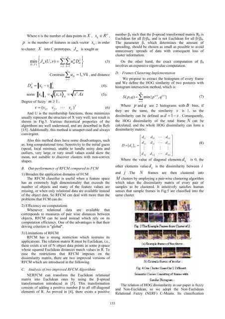
and j .The N frames are then clustered into
M clusters by employing a pair-wise clustering algorithm
which takes the dissimilarity matrix of every pair of
samples to be clustered. It intuitively satisfies human
senses that sample frames in Fig.5 are classified into the
same cluster.
The relation of HOG dissimilarity in our paper is fuzzy
and Non-Euclidean, so we adopt the Non-Euclidean
Relational Fuzzy (NERF) C-Means. Its classification
155