Download - Academy Publisher

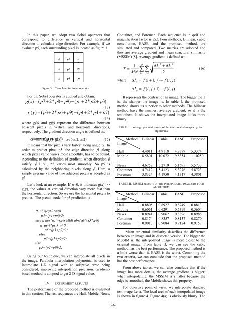
In this paper, we adopt two Sobel operators that
correspond to difference in vertical and horizontal
direction to calculate edge direction. For example, if we
evaluate p5, each surrounding pixel is located as figure 3.
Figure 3. Template for Sobel operator.
For p5, Sobel operator is applied and obtain:
gx () = ( p7+ 2* p8+ p9) − (1 p+ 2* p2+
p3)
(13)
gy ( ) = ( p3+ 2* p6+ p9) − ( p1+ 2* p4+
p7)
(14)
where g(x) and g(y) represent the difference between
adjacent pixels in vertical and horizontal directions,
respectively. The gradient direction angle is defined as:
α= arctan( gy ( )/ gx ( )) α∈(-π/2, π/2) (15)
It means that the pixels vary fastest along angle α . In
order to predict pixel p5, the edge direction β, along
which pixel value varies most smoothly, has to be found.
According to the definition of gradient, when direction β
satisfy β ⊥ α , p5 varies most smoothly. So p5 is
calculated by the neighboring pixels along β. Here, a
simple average value of two adjacent pixels is adopted as
p5.
Let’s look at an example. If α=0, it indicates g(x) >>
g(y), the values at vertical direction vary more fast than
the horizontal direction. So we use the horizontal pixels to
predict. The pseudo code for p5 prediction is
If abs(α)≤(π/8)
p5=(p4+p6)/2;
else if abs(α) >(π/8 )&& abs(α)≤(3*π/8)
if g(y)*g(x) ≥0
p5=(p3+p7)/2;
else
p5=(p1+p9)/2;
else
p5=(p2+p8)/2;
Using our technique, we can interpolate all pixels in
the image. Parabola interpolation polynomial is used to
interpolate 1-D signal with an adaptive error being
considered, improving interpolation precision. Gradientbased
method is adopted to get 2-D signal value.
IV. EXPERIMENT RESULTS
The performance of the proposed method is evaluated
in this section. The test sequences are Hall, Mobile, News,
Container, and Foreman. Each sequence is in qcif and
magnification factor is 2x2. Four methods, Bilinear, cubic
convolution, EASE, and the proposed method, are
simulated and compared. Two metrics are adopted and
they are average gradient and mean structural similarity
(MSSIM) [8]. Average gradient is defined as:
T
M N
1 Δ I +ΔI
MN = = 2
i 1 j 1
2 2
x y
= ∑∑ (16)
where Δ I = f ( i + 1, j) − f ( i, j)
x
Δ I = f(, i j+ 1) − f(, i j)
y
It represents the contrast of an image. The bigger the T
is, the sharper the image is. In table I, the proposed
method shows its superior to other methods. The bilinear
method have the smallest average gradient, so it is the
smoothest. It shows the interpolated image looks more
blurry.
TABLE I. average gradient results of the interpolated images by four
algorithms
Method
Image
Bilinear Cubic EASE Proposed
Hall 4.4011 4.9118 4.8379 5.3374
Mobile 8.5801 10.072 9.8354 11.0250
0
News 4.6758 5.2719 5.1695 5.5733
Container 4.7412 5.4123 5.3276 5.8723
Foreman 3.8324 4.1950 4.1317 4.3801
TABLE II. MSSIM RESULTS OF THE INTERPOLATED IMAGES BY FOUR
ALGORITHMS
Method
Image
Bilinear Cubic EASE Proposed
Hall 0.8805 0.8927 0.8749 0.8813
Mobile 0.6061 0.6291 0.5399 0.5604
News 0.8941 0.9062 0.8896 0.8988
Container 0.8174 0.8357 0.8137 0.8270
Foreman 0.9013 0.9084 0.9124 0.9157
Mean structural similarity describes the difference
between an image and its distorted version. The bigger the
MSSIM is, the interpolated image is more closer to the
original image. From table II, we can see the cubic
method has the best performance. The proposed method is
a little worse than it. EASE is the worst. Combining the
two criteria, we can conclude that the proposed method
has the best performance.
From above tables, we can also conclude that if the
image has more details, the average gradient is bigger;
when interpolating, the MSSIM is smaller because the
edge is smoothed, the Mobile shows this property.
For objective point of view, we interpolate standard
test image Lena. The local area of each interpolated image
is shown in figure 4. Figure 4(a) is obviously blurry. The
269