Download - Academy Publisher
Download - Academy Publisher
Download - Academy Publisher
You also want an ePaper? Increase the reach of your titles
YUMPU automatically turns print PDFs into web optimized ePapers that Google loves.
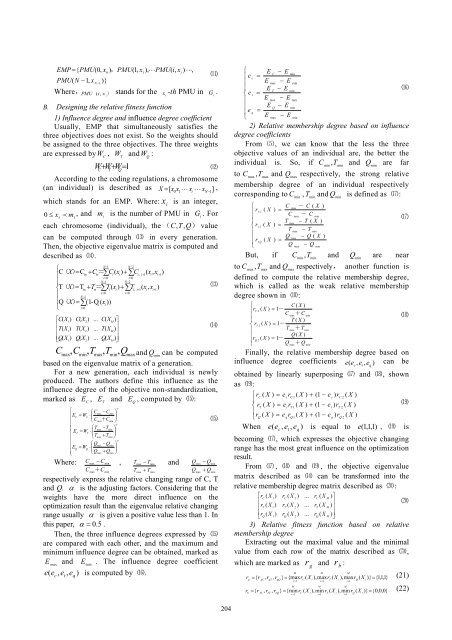
EMP = { PMU(0,<br />
x ),<br />
PMU(1,<br />
x ), ⋅⋅⋅PMU(<br />
i,<br />
x ) ⋅⋅⋅,<br />
0<br />
PMU(<br />
N −1,<br />
x )}<br />
N −1<br />
Where, PMU ( i,<br />
) stands for the x -th PMU in<br />
i<br />
x i<br />
1<br />
i<br />
⑾<br />
G .<br />
i<br />
B. Designing the relative fitness function<br />
1) Influence degree and influence degree coefficient<br />
Usually, EMP that simultaneously satisfies the<br />
three objectives does not exist. So the weights should<br />
be assigned to the three objectives. The three weights<br />
are expressed byW , W andW :<br />
C<br />
T<br />
W<br />
C+ WT<br />
+ WQ<br />
=1<br />
⑿<br />
According to the coding regulations, a chromosome<br />
(an individual) is described as X = [ x0x1<br />
⋅⋅⋅ x i<br />
⋅⋅⋅ xN<br />
−1]<br />
,<br />
which stands for an EMP. Where: x is an integer,<br />
0 ≤ xi p m i<br />
, and m<br />
i<br />
is the number of PMU in G<br />
i<br />
. For<br />
each chromosome (individual), the ( C , T,<br />
Q)<br />
value<br />
can be computed through ⒀ in every generation.<br />
Then, the objective eigenvalue matrix is computed and<br />
described as ⒁.<br />
N−1<br />
N−2<br />
⎧<br />
C( X)<br />
= Cin<br />
+ Ctr=<br />
+<br />
⎪<br />
∑C<br />
i(<br />
xi<br />
) ∑C<br />
i,<br />
i+<br />
1(<br />
xi<br />
, xi<br />
+ 1)<br />
i=<br />
0<br />
i=<br />
0<br />
⎪<br />
N−1<br />
N−2<br />
⎨T( X)<br />
= Tin<br />
+ Ttr=∑<br />
Ti<br />
( xi<br />
) + ∑T<br />
i,<br />
i+<br />
1(<br />
xi<br />
, xi<br />
+ 1)<br />
i=<br />
0<br />
i=<br />
0<br />
⎪<br />
N−1<br />
⎪Q( X)<br />
= ∑(1-Q i(<br />
xi<br />
))<br />
⎩<br />
i=<br />
0<br />
⎡C(<br />
X1)<br />
C(<br />
X2)<br />
... C(<br />
XM)<br />
⎤<br />
⎢<br />
⎥<br />
⎢<br />
T(<br />
X1)<br />
T(<br />
X2)<br />
... T(<br />
X )<br />
⒁<br />
M<br />
⎥<br />
⎢⎣<br />
Q(<br />
X ) ( ) ... ( ) ⎥<br />
1<br />
Q X2<br />
Q XM<br />
⎦<br />
Cmax , Cmin,<br />
Tmax,<br />
Tmin,<br />
Qmaxand Q min<br />
can be computed<br />
based on the eigenvalue matrix of a generation.<br />
For a new generation, each individual is newly<br />
produced. The authors define this influence as the<br />
influence degree of the objective non-standardization,<br />
marked as E , E and E , computed by ⒂:<br />
Where:<br />
C<br />
T<br />
Q<br />
Q<br />
i<br />
⒀<br />
α<br />
⎧ ⎛ C ⎞<br />
max<br />
−Cmin<br />
⎪E<br />
⎜<br />
⎟<br />
C<br />
= WC<br />
⋅<br />
⎪ ⎝ Cmax+ Cmin<br />
⎠<br />
⒂<br />
⎪<br />
α<br />
⎛T<br />
− ⎞<br />
max<br />
Tmin<br />
⎨ E = ⋅<br />
⎜<br />
⎟<br />
T<br />
WT<br />
⎪ ⎝Tmax<br />
+ Tmin<br />
⎠<br />
α<br />
⎪ ⎛ Q −Q<br />
⎞<br />
max min<br />
⎪E<br />
= W ⋅<br />
⎪<br />
⎜<br />
⎟<br />
Q Q<br />
⎩ ⎝ Q + Q<br />
max min ⎠<br />
C − C<br />
max min , T − T<br />
max min and Q − Q<br />
max min<br />
C +C<br />
T + T<br />
Q + Q<br />
max<br />
min<br />
respectively express the relative changing range of C, T<br />
and Q. α is the adjusting factors. Considering that the<br />
weights have the more direct influence on the<br />
optimization result than the eigenvalue relative changing<br />
range usually α is given a positive value less than 1. In<br />
this paper, α = 0. 5 .<br />
Then, the three influence degrees expressed by ⒂<br />
are compared with each other, and the maximum and<br />
minimum influence degree can be obtained, marked as<br />
E and E<br />
max<br />
min<br />
. The influence degree coefficient<br />
e e , e , e ) is computed by ⒃.<br />
(<br />
c t q<br />
max<br />
min<br />
max<br />
min<br />
⎧ E − E<br />
C min<br />
⎪ e =<br />
c<br />
⎪ E<br />
max<br />
− E<br />
min<br />
⎪ E − E<br />
⒃<br />
T min<br />
⎨ e<br />
t<br />
=<br />
⎪ E − E<br />
max<br />
min<br />
⎪ E − E<br />
Q min<br />
⎪ e<br />
q<br />
=<br />
⎩ E − E<br />
max<br />
min<br />
2) Relative membership degree based on influence<br />
degree coefficients<br />
From ⑸, we can know that the less the three<br />
objective values of an individual are, the better the<br />
individual is. So, if Cmin ,Tmin<br />
and Qmin<br />
are far<br />
to Cmax ,Tmax<br />
and Qmax<br />
respectively, the strong relative<br />
membership degree of an individual respectively<br />
corresponding to C min<br />
, Tmin<br />
and Q min<br />
is defined as ⒄:<br />
⎧<br />
C - C ( X )<br />
max<br />
⎪ r1<br />
C<br />
( X ) =<br />
⎪<br />
C - C<br />
max<br />
min<br />
⒄<br />
⎪<br />
T − T ( X )<br />
max<br />
⎨ r ( X ) =<br />
1 T<br />
⎪<br />
T − T<br />
max<br />
min<br />
⎪<br />
Q − Q ( X )<br />
max<br />
⎪<br />
r ( X ) =<br />
1 Q<br />
⎩<br />
Q − Q<br />
max<br />
min<br />
But, if Cmin,Tmin<br />
and Qmin<br />
are near<br />
to Cmax,Tmax<br />
and Q max<br />
respectively, another function is<br />
defined to compute the relative membership degree,<br />
which is called as the weak relative membership<br />
degree shown in ⒅:<br />
⎧<br />
C ( X )<br />
⎪rC<br />
2<br />
( X ) = 1-<br />
⎪<br />
C +C<br />
max min<br />
⒅<br />
⎪<br />
T ( X )<br />
⎨ r ( X ) = 1-<br />
T 2<br />
⎪<br />
T +T<br />
max min<br />
⎪<br />
Q(<br />
X )<br />
⎪<br />
r ( X ) = 1-<br />
Q 2<br />
⎩<br />
Q +Q<br />
max min<br />
Finally, the relative membership degree based on<br />
influence degree coefficients e ( ec<br />
, et<br />
, eq<br />
) can be<br />
obtained by linearly superposing ⒄ and ⒅, shown<br />
as ⒆:<br />
⎧ r ( X ) = e r ( X ) + (1 − e ) r ( X )<br />
C<br />
c C 1<br />
c C 2<br />
⎪<br />
⎨ r ( X ) = e r<br />
1<br />
( X ) + (1 − e ) r<br />
2<br />
( X )<br />
⒆<br />
T<br />
t T<br />
t T<br />
⎪<br />
⎩r<br />
( X ) = e r ( X ) + (1 − e ) r ( X )<br />
Q<br />
q Q 1<br />
q Q 2<br />
When e ( ec,<br />
et<br />
, eq<br />
) is equal to e (1,1,1 ) , ⒆ is<br />
becoming ⒄, which expresses the objective changing<br />
range has the most great influence on the optimization<br />
result.<br />
From ⒄ , ⒅ and ⒆ , the objective eigenvalue<br />
matrix described as ⒁ can be transformed into the<br />
relative membership degree matrix described as ⒇:<br />
⎡r<br />
( X ) r ( X ) ... r ( X ) ⎤<br />
C 1 C 2<br />
C M<br />
⎢<br />
⎥<br />
⒇<br />
⎢r<br />
( X ) r ( X ) ... r ( X )<br />
T 1 T 2<br />
T M ⎥<br />
⎢<br />
⎥<br />
⎣r<br />
( X ) r ( X ) ... r ( X )<br />
Q 1 Q 2<br />
Q M ⎦<br />
3) Relative fitness function based on relative<br />
membership degree<br />
Extracting out the maximal value and the minimal<br />
value from each row of the matrix described as ⒇,<br />
which are marked as r and r b<br />
:<br />
g<br />
M<br />
M<br />
M<br />
r = { r , r , r } = {maxr<br />
( X ),maxr<br />
( X ),maxr<br />
( X )} = {1,1,1} (21)<br />
g<br />
gC<br />
gT<br />
gQ<br />
i=<br />
1<br />
C<br />
i<br />
i=<br />
1<br />
r = { r , r , r<br />
M<br />
M<br />
M<br />
} = {min r ( X ), min r ( X ), min r ( X )} = {0,0,0} (22)<br />
b<br />
bC<br />
bT<br />
bQ<br />
i=<br />
1<br />
C<br />
i<br />
i=<br />
1<br />
T<br />
T<br />
i<br />
i<br />
i=<br />
1<br />
i=<br />
1<br />
Q<br />
Q<br />
i<br />
i<br />
204


