Download - Academy Publisher

( n + 1)
f ( ξ )
Rn( x) = f ( x) − Ln( x) = ω
n+
1( x)
( n + 1)!
where ξ∈ [a, b], and
n 1 0 1
(2)
ω +
( x) = ( x− x )( x− x )...( x− x ) (3)
In fact, the n+1 order derivative of image function f(x)
is unavailable and it has to be replaced. It is well known
that adjacent pixels always have similar property and
errors are closely related to each other. Based on this
observation, we propose an error estimation which will
be discussed in section Ⅲ.
III. THE PROPOSED INTERPOLATION ALGORITHM
For a typical image expansion, for example the
magnification factor is 2x2, an image of NxM pixels is
expanded to high resolution 2Nx2M. We can get arbitrary
high resolution image by changing polynomial coefficient
in (1). Two steps are processed to implement 1-D and 2-D
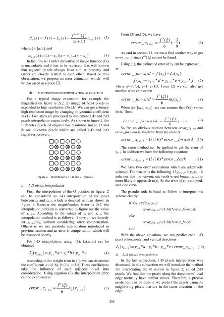
pixels interpolation respectively. As shown in figure 2, the
denotes pixels of original low resolution image, Օ and
⊗ are unknown pixels which are called 1-D and 2-D
signal respectively.
Figure 2. Distribution of 1-D and 2-D pixels
A. 1-D pixels interpolation
First, the interpolation of the Օ position in figure. 2
can be considered as 1-D interpolation of the pixel
between x k and x k+1 , which is denoted as x, as shown in
figure 1. Because the magnification factor is 2x2, the
interpolation problem is converted to figure out the value
of x k+1/2 . According to the values of x k and x k+1 , the
interpolation method is as follows. If y k =y k+1 , we directly
let y k+1/2 =y k , without considering error compensation.
Otherwise we use parabola interpolation introduced in
previous section and an error is compensation which will
be discussed shortly.
For 1-D interpolation, using (1), L 2 (x k+1/2 ) can be
obtained
L ( x ) = y * a+ y * b+ y * c (4)
2 k+ 1/2 k− 1 k k+
1
According to the weight term in (1), we can determine
the coefficients a=-(1/8), b=3/4, c=3/8. These coefficients
take the influence of each adjacent pixel into
consideration. Using equation (2), the interpolation error
can be expressed as
3
f ( ξ )
error _ xk+ 1/2
= ω
3( xk+
1/2)
(5)
6
n
From (3) and (5), we have:
3
f ( ξ ) 3
error _ xk
+ 1/2
= ( − ) (6)
6 8
As said in section II, we must find another way to get
error_x k+1/2 since f (3) ( ξ) cannot be found.
Using (1), the estimated error of x k can be expressed
as :
error _ forward = f ( xk) − L2
( xk)
= f ( xk) − yk−2* d + yk− 1* e+ yk+
1*
f (7)
where d=-(1/3), e=1, f=1/3. From (2) we can also get
another error expression
3
f (1) ξ
error _ forward ω
3( xk
)
6
= (8)
When ξ∈ [x k-2 , x k+2 ], we can assume that f 3 (ξ) varies
little. Then:
f
3 ( ξ )
error _ forw ard = ( − 2) (9)
6
So far, an obvious relation between error_x k+1/2 and
error_forward is available from (6) and (9):
error _ xk
+ 1/2
= (3/16)* error _ forward (10)
The same method can be applied to get the error of
y k+1 . In addition we have the following equation:
error _ xk
+ 1/2
= (3/16)* error _ back (11)
We have two error evaluations which are adaptively
selected. The reason is the following. If y k+1 -yk≥y k -y k-1 , it
indicates that the varying rate tends to get bigger, y k+1/2 is
more likely to approach to y k . So the error of y k is adopted,
and vice versa.
The pseudo code is listed as follow to interpret this
scheme clearly:
If (y k+1 -y k ≥y k -y k-1 )
error_x k+1/2 =(3/16)*error_forward;
else
error_x k+1/2 =(3/16)*error_back;
end
With the above equations, we can predict each 1-D
pixel at horizontal and vertical directions
L ( x ) = y * a+ y * b+ y * c+ error _ x (12)
2 k+ 1/2 k− 1 k k+ 1 k+
1/2
B. 2-D pixels interpolation
In the last subsection, 1-D pixels interpolation was
discussed. In this subsection we will introduce the method
for interpolating the ⊗ shown in figure 2, called 2-D
pixels. We find that the pixels along the direction of local
edge normally have similar values. Therefore, a precise
prediction can be done if we predict the pixels using its
neighboring pixels that are in the same direction of the
edge.
268