Download - Academy Publisher

In order to reduce to the number of textures and to
switch computational domain quickly, 16 textures are
used to store interior stress-velocity parameters, called
whole- texture with the size width*height, width and
height denoting grid-point numbers in x and z direction
respectively. It equals the size of the rendering viewport.
The input seismic parameters Vp, Vs, Qp, Qs, ρ are also
stored in whole- texture. 5*2 extra textures, called x-
direction-texture, are used to express all velocity and
stress parameters in x absorbing direction; and the size of
each texture is (2*NBC, height), NBC defining the
gridpoints of the absorbing boundary. In our work, NBC
is 10. Simultaneously, there are 5*2 extra arrays in z
absorbing direction, called z-direction-texture, and the
size is (width, 2*NBC).There are actually another 20
arrays at time t+1.
From above analysis, the memory requirements
MEMREq for 2D viscoelastic modelling is obtained by,
2
2
MEMREg = ( N ∗C
+ N * NBC * D)
∗ Fz /1024 (11)
where the total number C of the whole-texture is 21
and the total number D of x-and z- direction- texture is 40.
Fz of float size equals 4 bytes.
TABLE I
MEMORY REQUIREMENTS FOR 2D VISCOELASTIC MODEL
Gridsize( N 2 ) Memory Requirements
512 2 22.56M
1024 2 87.12 M
2048 2 342.25 M
4096 2 1356.50 M
Table1 shows 2D viscoelastic model which is only less
than 2048*2048 gridsizes can be supported on current
GPUs directly, since graphics video memory size is about
256-512M in general.
D. Fragment processing
The results of each step are written to a twodimensional
memory location called framebuffer. But the
characteristics of the GPU prohibit the usage of the buffer
for reading and writing operations at the same time.
Fortunately, the OpenGL extension FrameBuffer Object
(FBO) allows reusing the framebuffer content as a texture
for further processing in a subsequent rendering pass and
the “ping-pong" method allows two buffers swap their
role after each write operation [3]. In order to generate
and store intermediate results for each simulating step on
GPUs, our strategy is to bind each texture that is rendered
to onto one attachment on an assigned FBO; two textures
binding on the same FBO are used to represent one
stress-velocity component at time t and t+1, respectively.
After each frame, FBO attachments are swapped and the
latest updated textures are then used as inputs for the next
simulation step while N = 1- N (N = 0, 1).
IV. NUMERICAL EXAMPLES
We have experimented with our GPU accelerated
method implemented using C++/OpenGL and Cg shader
language on a PC with Intel Core(TM)2 Duo E7400
2.8GHz, 2G main memory. The graphics chip is NVidia
GeForce 9800GT with 512M video memory and 550MHz
core frequency. The OS is Windows XP. All the results
related to the GPU are based on 32-bit single-precision
computation of the rendering pipeline. For comparison,
we have also implemented a software version of the
seismic simulation using single-precision floating point,
and we have measured their performance on the same
machine.
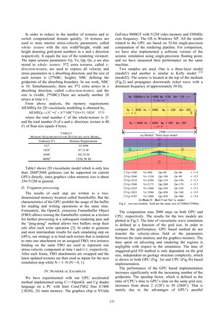
Two samples are used. One is a three-layer model
(model1) and another is similar to Kelly model [14]
(model2). The source is located at the top of the medium
(Fig.2) and propagates downwards ricker wave with a
dominant frequency of approximately 50 Hz.
Vp =2600m/s Vs =1800 Qp =120 Qs= 110 ρ=
2 4g/cm 3
Vp = 3050 Vs = 2400 Qp = 230 Qs= 220
ρ= 2 7
Vp = 4000 Vs = 3300 Qp = 350 Qs= 267
ρ=3 0
2500
(a) Model1: Three layer model
1
2
4
3
5
6
7
2500
m
1Vp=1200 Vs=800 Qp=80 Qs=60 ρ=1.4
2Vp=2440
Vs=1330 Qp=100 Qs=90 ρ=2.2
3Vp=3210 Vs=2389 Qp=219 Qs=190 ρ=2.3
4Vp=3500 Vs=2173 Qp=200 Qs=170 ρ=2.5
5Vp=3225 Vs=1800 Qp=294 Qs=220 ρ=2.5
6Vp=3822 Vs=2980 Qp=490 Qs=340 ρ=2.6
7Vp=4785 Vs=3800 Qp=450 Qs=400 ρ=3.4
(b) Model2: Modified Kelly model
Fig.2. two test models: both are the same size of 2500m*2500m.
The computation runs 2000 steps on both GPU and
CPU, respectively. The results for the two models are
plotted in Fig.3. The time of viscoelastic wave simulation
is defined as a function of the grid size. In order to
compare the performance, GPU based method do not
transfer the velocity-stress field or the parameters
between the main memory and the graphics memory. The
time spent on advecting and rendering the regions is
negligible with respect to the simulation. The time of
staggered-grid FD method is only dependent on the grid
size, independent on geology structure complexity, which
is shown in both GPU (Fig. 3a) and CPU (Fig.3b) based
implementation.
The performance of the GPU based implementation
increases significantly with the increasing number of the
gridpoints. The speedup factor, which is defined as the
ratio of CPU’s time to GPU’s time on the same grid size,
increases from about 2 (128 2 ) to 50 (2048 2 ). That is
mainly due to the advantages of GPU’s parallel
131