Download - Academy Publisher

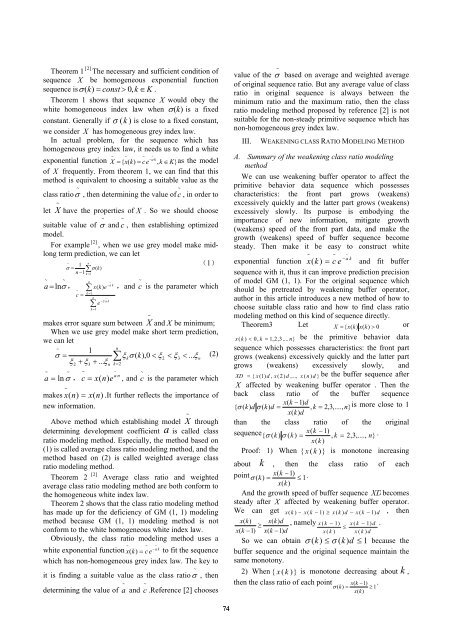
Theorem 1 [ 2]
The necessary and sufficient condition of
sequence X be homogeneous exponential function
sequence isσ ( k)
= const > 0,
k ∈ K .
Theorem 1 shows that sequence X would obey the
white homogeneous index law when σ(k)
is a fixed
constant. Generally if σ (k ) is close to a fixed constant,
we consider X has homogeneous grey index law.
In actual problem, for the sequence which has
homogeneous grey index law, it needs us to find a white
~ ~ ~ ~
−a k
exponential function X = { x(
k)
= ce , k ∈ K}
as the model
of X frequently. From theorem 1, we can find that this
method is equivalent to choosing a suitable value as the
class ratio ~ σ , then determining the value of c ~ , in order to
~
let X have the properties of X . So we should choose
suitable value of ~ σ and c ~ , then establishing optimized
model.
For example [ 2]
, when we use grey model make midlong
term prediction, we can let
~
n
(1)
σ = ∑σ
( k)
~
~
a = lnσ ,
1
1
n − k=
2
n
∑
x
~
k = 1
c =
n
∑
k = 1
~
−a k
( k)
e ,and c ~ is the parameter which
e
~
−2
a k
~
makes error square sum between X and X be minimum;
When we use grey model make short term prediction,
we can let
~
n
σ = 1
∑ ξ
kσ
( k),0
< ξ ξ ξ
n
ξ ξ ... ξ
...
2
<
3
< (2)
+ +
2
3
n k=
2
~ ~ ~ ~
~
a n
a = lnσ , c = x(
n)
e , and c is the parameter which
~
(
makes x n)
= x(
n)
.It further reflects the importance of
new information.
~
Above method which establishing model X through
determining development coefficient a is called class
ratio modeling method. Especially, the method based on
(1) is called average class ratio modeling method, and the
method based on (2) is called weighted average class
ratio modeling method.
[2]
Theorem 2 Average class ratio and weighted
average class ratio modeling method are both conform to
the homogeneous white index law.
Theorem 2 shows that the class ratio modeling method
has made up for the deficiency of GM (1, 1) modeling
method because GM (1, 1) modeling method is not
conform to the white homogeneous white index law.
Obviously, the class ratio modeling method uses a
~ ~ ~
−a
k
white exponential function x(
k)
= c e to fit the sequence
which has non-homogeneous grey index law. The key to
it is finding a suitable value as the class ratio ~ σ , then
determining the value of ~ a and ~ c .Reference [2] chooses
value of the ~ σ based on average and weighted average
of original sequence ratio. But any average value of class
ratio in original sequence is always between the
minimum ratio and the maximum ratio, then the class
ratio modeling method proposed by reference [2] is not
suitable for the non-steady primitive sequence which has
non-homogeneous grey index law.
III. WEAKENING CLASS RATIO MODELING METHOD
A. Summary of the weakening class ratio modeling
method
We can use weakening buffer operator to affect the
primitive behavior data sequence which possesses
characteristics: the front part grows (weakens)
excessively quickly and the latter part grows (weakens)
excessively slowly. Its purpose is embodying the
importance of new information, mitigate growth
(weakens) speed of the front part data, and make the
growth (weakens) speed of buffer sequence become
steady. Then make it be easy to construct white
~
−a k
exponential function x(
k ) = c e and fit buffer
sequence with it, thus it can improve prediction precision
of model GM (1, 1). For the original sequence which
should be pretreated by weakening buffer operator,
author in this article introduces a new method of how to
choose suitable class ratio and how to find class ratio
modeling method on this kind of sequence directly.
Theorem3 Let X = { x(
k)
x(
k)
> 0 or
x ( k ) < 0, k = 1,2,3.... n}
be the primitive behavior data
sequence which possesses characteristics: the front part
grows (weakens) excessively quickly and the latter part
grows (weakens) excessively slowly, and
XD = { x (1) d , x (2) d ,..., x ( n ) d } be the buffer sequence after
X affected by weakening buffer operator . Then the
back class ratio of the buffer sequence
x(
k −1)
d
{ σ ( k ) d σ ( k)
d = , k = 2,3,...., n}
is more close to 1
x(
k)
d
than the class ratio of the original
sequence x(
k − 1)
{ σ ( k ) σ ( k ) = , k = 2,3,...., n
x(
k )
} .
Proof: 1) When { x ( k )} is monotone increasing
about k , then the class ratio of each
point x(
k −1)
σ ( k)
= ≤ 1.
x(
k)
And the growth speed of buffer sequence XD becomes
steady after X affected by weakening buffer operator.
We can get
, then
x ( k ) − x ( k − 1) ≥ x ( k ) d − x ( k − 1)
d
x(
k)
x(
k)
d
≥ , namely x ( k − 1) x ( k − 1) d .
≤
x(
k −1)
x(
k −1)
d
x ( k ) x ( k ) d
So we can obtain σ ( k)
≤ σ ( k)
d ≤ 1 because the
buffer sequence and the original sequence maintain the
same monotony.
2) When { x ( k )} is monotone decreasing about k ,
then the class ratio of each point x(
k −1)
.
~
~
σ ( k)
= ≥ 1
x(
k)
74