Cálculo e Estimação de Invariantes Geométricos: Uma ... - Impa

More documents

Recommendations

Info

50 3.5. Segunda Forma Fundamental Exemplo 3.28. Seja P = {(x, y, z) ∈ R 3 /ax + by + cz + d = 0} um plano. O vetor normal em p ∈ P é dado por N = e é constante, logo dNp = 0. 1 √ (a, b, c) a2 + b2 + c2 Exercício 3.29. Mostre que a aplicação dNp é auto-adjunta, isto é 〈dNpv, w〉 = 〈v, dNpw〉. Definição 3.30. Seja p ∈ S e seja dNp : TpS → TpS a diferencial da aplicação de Gauss. O determinante de dNp é chamado curvatura Gaussiana K de S em p. A metade do traço de dNp é chamado de curvatura média H de S em p. Definição 3.31. A forma quadrática IIp : TpS × TpS → R, definida em TpS por IIp(v) = −〈dNp(v), v〉 é chamada segunda forma fundamental de S em p. Vamos escrever a expressão da segunda forma fundamental na base {σu, σv}. Seja α(t) = σ(u(t), v(t)) uma curva parametrizada em S, com σ(0) = p. O vetor tangente a α(t) em p é α ′ (t) = σuu ′ + σvv ′ e a diferencial da aplicação de Gauss Portanto, onde dN(α ′ ) = N ′ (u(t), v(t)) = Nuu ′ + Nvv ′ . IIp(α ′ ) = −〈dNp(α ′ ), α ′ 〉 = −〈Nuu ′ + Nvv ′ , σuu ′ + σvv ′ 〉 = eu ′2 + 2fu ′ v ′ + gv ′2 , e = −〈Nu, σu〉, f = −〈Nv, σv〉 e g = −〈Nv, σv〉. Os coeficientes e, f e g são chamados coeficientes da segunda forma fundamental.
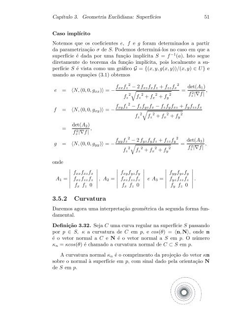
Capítulo 3. Geometria Euclidiana: Superfícies 51 Caso implícito Notemos que os coeficientes e, f e g foram determinados a partir da parametrização σ de S. Podemos determiná-los no caso em que a superfície é dada por uma função implícita S = f −1 (a). Isto segue diretamente do teorema da função implícita, pois localmente a superfície S é vista como um gráfico G = {(x, y, g(x, y))/(x, y) ∈ U} e usando as equações (3.1) obtemos e = 〈N, (0, 0, gxx)〉 = − fxxfz 2 − 2 fxzfxfz + fzzfx 2 � fz 2 fz 2 + fx 2 + fy 2 = det(A1) f 2 z |∇f| , f = 〈N, (0, 0, gxy)〉 = − fxyfz 2 − fzfyzfx − fzfyfxz + fyfzzfx � = det(A2) f 2 z |∇f| , fz 2 fz 2 + fx 2 + fy 2 g = 〈N, (0, 0, gyy)〉 = − fyyfz 2 − 2 fyzfyfz + fzzfy 2 � onde � � � A1 = � � � fxxfxzfx fxzfzzfz fx fz 0 3.5.2 Curvatura � � � � � � , A2 � � � = � � � fz 2 fxyfyzfy fxzfzzfz fx fz 0 fz 2 + fx 2 + fy 2 � � � � � � e A3 � � � = � � � fyyfyzfy fyzfzzfz fy fz 0 = det(A3) f 2 z |∇f| , Daremos agora uma interpretação geométrica da segunda forma fundamental. Definição 3.32. Seja C uma curva regular na superfície S passando por p ∈ S, κ a curvatura de C em p, e cos(θ) = 〈n, N〉, onde n é o vetor normal a C e N é o vetor normal a S em p. O número κn = κcos(θ) é chamado a curvatura normal de C ⊂ S em p. A curvatura normal κn é o comprimento da projeção do vetor κn sobre o normal à superfície em p, com sinal dado pela orientação N de S em p. � � � � � � .
Page 1:
Cálculo e Estimação de Invariant
Page 4 and 5: Copyright © 2011 by M. Andrade e T
Page 7 and 8: Sumário 1 Introdução 7 1.1 Objet
Page 9: Sumário 5 5.3 Interpretação Geom
Page 12 and 13: 8 1.1. Objetos Geométricos Este li
Page 14 and 15: 10 1.3. Contextos de Modelagem 1.3
Page 16 and 17: 12 1.4. Técnicas de Mudança de Co
Page 19 and 20: Capítulo 2 Geometria Euclidiana: C
Page 21 and 22: Capítulo 2. Geometria Euclidiana:
Page 33: Capítulo 2. Geometria Euclidiana:
Page 36 and 37: 32 3.1. Modelos Euclidianos de Supe
Page 44 and 45: 40 3.2. Mudança de Contextos Estas
Page 46 and 47: 42 3.2. Mudança de Contextos Figur
Page 48 and 49: 44 3.3. Plano Tangente; Vetor Norma
Page 50 and 51: 46 3.4. Primeira Forma Fundamental
Page 52 and 53: 48 3.4. Primeira Forma Fundamental
Page 56 and 57: 52 3.5. Segunda Forma Fundamental $
Page 58 and 59: 54 3.5. Segunda Forma Fundamental 3
Page 60 and 61: 56 3.5. Segunda Forma Fundamental C
Page 62 and 63: 58 3.5. Segunda Forma Fundamental 3
Page 64 and 65: 60 3.6. Discussão perfície discre
Page 66 and 67: 62 4.1. Invariância Afim Definiç
Page 68 and 69: 64 4.1. Invariância Afim Cônicas
Page 70 and 71: 66 4.2. Modelos de Curvas 4.2 Model
Page 72 and 73: 68 4.2. Modelos de Curvas xi+1 zi F
Page 74 and 75: 70 4.3. Curvas Paramétricas Logo,
Page 76 and 77: 72 4.3. Curvas Paramétricas '"#$%
Page 78 and 79: 74 4.3. Curvas Paramétricas Portan
Page 80 and 81: 76 4.3. Curvas Paramétricas Propos
Page 82 and 83: 78 4.3. Curvas Paramétricas O pont
Page 84 and 85: 80 4.4. Curvas Implícitas 4.4.1 Ex
Page 86 and 87: 82 4.5. Discussão 4.4.3 Fórmulas
Page 89 and 90: Capítulo 5 Geometria Afim: Superf
Page 91 and 92: Capítulo 5. Geometria Afim: Superf
Page 105 and 106:
Capítulo 5. Geometria Afim: Superf
Page 107 and 108:
Page 109 and 110:
Page 111 and 112:
Page 113 and 114:
Page 115 and 116:
Page 117 and 118:
Page 120 and 121:
116 5.7. Discussão Figura 5.13: Me
Page 122 and 123:
118 6.1. Problemas Discretos tal
Page 124 and 125:
120 6.3. Desafios Atuais 6.3 Desafi
Page 126 and 127:
122 Referências Bibliográficas [C
Page 128 and 129:
124 Referências Bibliográficas [M
Page 131:
Índice Remissivo Área, 48 Aplica
show all

Cálculo e Estimação de Invariantes Geométricos: Uma ... - Impa

Create successful ePaper yourself

Delete template?

Save as template?