Handbook of Propagation Effects for Vehicular and ... - Courses

6-12
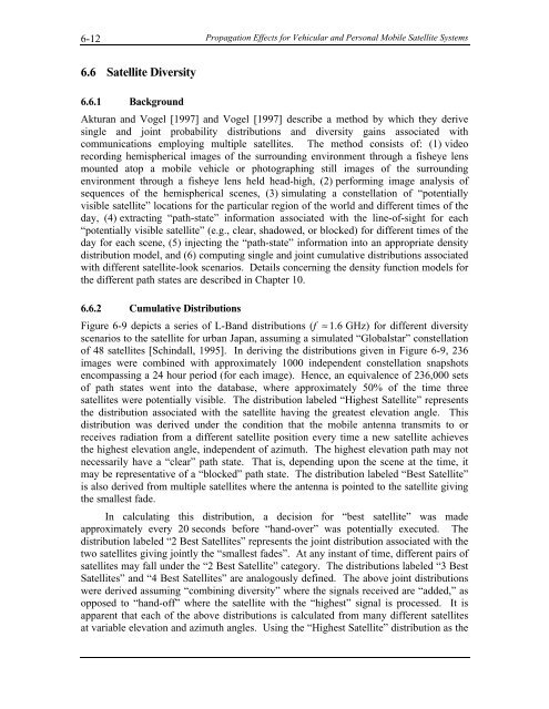
6.6 Satellite Diversity
6.6.1 Background
Propagation Effects for Vehicular and Personal Mobile Satellite Systems
Akturan and Vogel [1997] and Vogel [1997] describe a method by which they derive
single and joint probability distributions and diversity gains associated with
communications employing multiple satellites. The method consists of: (1) video
recording hemispherical images of the surrounding environment through a fisheye lens
mounted atop a mobile vehicle or photographing still images of the surrounding
environment through a fisheye lens held head-high, (2) performing image analysis of
sequences of the hemispherical scenes, (3) simulating a constellation of “potentially
visible satellite” locations for the particular region of the world and different times of the
day, (4) extracting “path-state” information associated with the line-of-sight for each
“potentially visible satellite” (e.g., clear, shadowed, or blocked) for different times of the
day for each scene, (5) injecting the “path-state” information into an appropriate density
distribution model, and (6) computing single and joint cumulative distributions associated
with different satellite-look scenarios. Details concerning the density function models for
the different path states are described in Chapter 10.
6.6.2 Cumulative Distributions
Figure 6-9 depicts a series of L-Band distributions (f ≈ 1.6 GHz) for different diversity
scenarios to the satellite for urban Japan, assuming a simulated “Globalstar” constellation
of 48 satellites [Schindall, 1995]. In deriving the distributions given in Figure 6-9, 236
images were combined with approximately 1000 independent constellation snapshots
encompassing a 24 hour period (for each image). Hence, an equivalence of 236,000 sets
of path states went into the database, where approximately 50% of the time three
satellites were potentially visible. The distribution labeled “Highest Satellite” represents
the distribution associated with the satellite having the greatest elevation angle. This
distribution was derived under the condition that the mobile antenna transmits to or
receives radiation from a different satellite position every time a new satellite achieves
the highest elevation angle, independent of azimuth. The highest elevation path may not
necessarily have a “clear” path state. That is, depending upon the scene at the time, it
may be representative of a “blocked” path state. The distribution labeled “Best Satellite”
is also derived from multiple satellites where the antenna is pointed to the satellite giving
the smallest fade.
In calculating this distribution, a decision for “best satellite” was made
approximately every 20 seconds before “hand-over” was potentially executed. The
distribution labeled “2 Best Satellites” represents the joint distribution associated with the
two satellites giving jointly the “smallest fades”. At any instant of time, different pairs of
satellites may fall under the “2 Best Satellite” category. The distributions labeled “3 Best
Satellites” and “4 Best Satellites” are analogously defined. The above joint distributions
were derived assuming “combining diversity” where the signals received are “added,” as
opposed to “hand-off” where the satellite with the “highest” signal is processed. It is
apparent that each of the above distributions is calculated from many different satellites
at variable elevation and azimuth angles. Using the “Highest Satellite” distribution as the