Handbook of Propagation Effects for Vehicular and ... - Courses

Signal Degradation for Line-of-Sight Communications 4-5
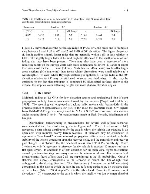
Table 4-2: Coefficients a, b in formulation (4-1) describing best fit cumulative fade
distributions for multipath in mountainous terrain.
Frequency Elevation = 30° Elevation = 45°
(GHz) a b dB Range a b dB Range
0.870 34.52 1.855 2-7 31.65 2.464 2-4
1.5 33.19 1.710 2-8 39.95 2.321 2-5
Figure 4-2 shows that over the percentage range of 1% to 10%, the fades due to multipath
vary between 2 and 5 dB at 45° and 2 and 8 dB at 30° elevation. The higher frequency
(L-Band) exhibits slightly larger fades that are generally within 1 dB or less relative to
UHF. The slightly larger fades at L-Band might be attributed to the small amount of tree
fading that may have been present. There may also have been a presence of more
reflecting facets on the canyon walls with sizes comparable to 20 cm (L-Band) or larger
than does exist for the UHF case (34 cm). Such facets (L-Band case) would offer larger
cross sections (Mie scattering) than facets whose dimensions were small relative to a
wavelength (UHF case) where Rayleigh scattering is applicable. Larger fades at the 30°
elevation relative to 45° may be attributed to some tree shadowing. It also may be
attributed to the fact that multipath is dominated by illuminated surfaces closer to the
vehicle; this implies lower reflecting heights and more shallow elevation angles.
4.2.2 Hilly Terrain
Multipath fading at 1.5 GHz for low elevation angles and unshadowed line-of-sight
propagation in hilly terrain was characterized by the authors [Vogel and Goldhirsh,
1995]. The receiving van employed a tracking helix antenna with beamwidths in the
principal planes of approximately 36° (i.e., ± 18° about the geometric axis). CW signals
from INMARSAT’s geostationary satellite MARECS B-2 were received at elevation
angles ranging from 7° to 14° for measurements made in Utah, Nevada, Washington and
Oregon.
Distributions corresponding to measurements for several well-defined scenarios
were executed and the results are given in Figure 4-3. Curve 1 (elevation = 14°)
represents a nine-minute distribution for the case in which the vehicle was standing in an
open area with minimal nearby terrain features. It therefore may be considered to
represent a “benchmark” where minimal propagation effects are combined with the
stability of the system dependent upon the receiver noise, and the transmitter and receiver
gain changes. It is observed that the fade level is less than 1 dB at 1% probability. Curve
2 (elevation = 14°) represents a reference for the vehicle in motion (12 minute run) in a
flat open terrain. In additions to effects described for the static case, signal fluctuations
caused by antenna tracking errors may also have been introduced here. For the open field
measurements, fades of less than 2 dB are experienced at the 1% probability. Curve 3
(labeled best aspect) corresponds to the scenario in which the line-of-sight was
orthogonal to the driving direction. This distribution (17 minute run at 14° elevation)
corresponds to the case in which the satellite and reflecting surfaces are on the same side
of the vehicle (labeled “Best Aspect”). On the other hand, Curve 4 (10 minute run at
elevation = 10°) corresponds to the case in which the satellite was (on average) ahead of