Handbook of Propagation Effects for Vehicular and ... - Courses
Handbook of Propagation Effects for Vehicular and ... - Courses
Handbook of Propagation Effects for Vehicular and ... - Courses
Create successful ePaper yourself
Turn your PDF publications into a flip-book with our unique Google optimized e-Paper software.
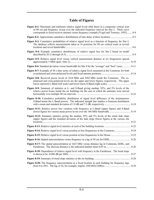
Table <strong>of</strong> Figures<br />
Figure 8-1: Maximum <strong>and</strong> minimum relative signal levels (thin lines) in a composite vertical scan<br />
<strong>of</strong> 80 cm <strong>and</strong> frequency sweep over the indicated frequency interval <strong>for</strong> Site 2. Thick curve<br />
corresponds to fixed receiver antenna versus frequency example [Vogel <strong>and</strong> Torrence, 1993]........ 8-4<br />
Figure 8-2: Approximate cumulative distributions <strong>of</strong> time delay at three locations. ................................ 8-5<br />
Figure 8-3: Cumulative probabilities <strong>of</strong> relative signal level as a function <strong>of</strong> frequency <strong>for</strong> Site 2.<br />
The database reflects measurements taken at 16 positions <strong>for</strong> 80 cm vertical scans at several<br />
locations <strong>and</strong> seven b<strong>and</strong>widths .................................................................................................... 8-6<br />
Figure 8-4: Example cumulative distributions <strong>of</strong> relative signal loss <strong>for</strong> Site 2 based on model<br />
described by (8-1) through (8-3). .................................................................................................. 8-9<br />
Figure 8-5: Relative signal level versus vertical measurement distance at six frequencies spaced<br />
approximately 5 MHz apart. (Site 2). .......................................................................................... 8-10<br />
Figure 8-6: St<strong>and</strong>ard deviation versus b<strong>and</strong>width <strong>for</strong> Site 4 <strong>for</strong> the “average” <strong>and</strong> “best” cases............. 8-11<br />
Figure 8-7: Example <strong>of</strong> 50 s time series <strong>of</strong> relative signal level measured at the Commons <strong>for</strong> both<br />
co-polarized <strong>and</strong> cross-polarized levels <strong>and</strong> fixed antenna positions............................................. 8-14<br />
Figure 8-8: Received power levels at 1618 MHz <strong>and</strong> 2492 MHz inside the Commons. The copolarized<br />
<strong>and</strong> cross-polarized levels are the upper <strong>and</strong> lower figures, respectively. The upper<br />
traces represent L-B<strong>and</strong> (left scale) <strong>and</strong> lower traces S-B<strong>and</strong> (right scale).................................... 8-15<br />
Figure 8-9: Summary <strong>of</strong> statistics at L- <strong>and</strong> S-B<strong>and</strong> giving median, 95%, <strong>and</strong> 5% levels <strong>of</strong> the<br />
relative power losses inside the six buildings <strong>for</strong> the case in which the antennas were moved<br />
horizontally over multiple 80 cm intervals. ................................................................................. 8-16<br />
Figure 8-10: Cumulative probability distribution <strong>of</strong> signal level difference <strong>of</strong> the instantaneous<br />
S-B<strong>and</strong> minus the L-B<strong>and</strong> powers. The indicated straight line implies a Gaussian distribution<br />
with a mean <strong>and</strong> st<strong>and</strong>ard deviation <strong>of</strong> 1.9 dB <strong>and</strong> 7.2 dB, respectively........................................ 8-18<br />
Figure 8-11: Relative power loss variation with frequency at L-B<strong>and</strong> (upper figure) <strong>and</strong> S-B<strong>and</strong><br />
(lower figure) <strong>for</strong> various mean power levels over the 160 MHz b<strong>and</strong>width................................. 8-19<br />
Figure 8-12: Summary statistics giving the median, 95% <strong>and</strong> 5% levels <strong>of</strong> the mean fade slope<br />
(upper figure) <strong>and</strong> the st<strong>and</strong>ard deviation <strong>of</strong> the fade slope (lower figure) at the various site<br />
locations..................................................................................................................................... 8-21<br />
Figure 8-13: Relative signal level statistics at each <strong>of</strong> the building locations. ....................................... 8-23<br />
Figure 8-14: Relative signal level versus position at four frequencies in the Commons......................... 8-24<br />
Figure 8-15: Relative signal level versus position at four frequencies in the House............................... 8-25<br />
Figure 8-16: Spatial autocorrelation versus frequency at a lag <strong>of</strong> 50 cm <strong>for</strong> EERL................................ 8-26<br />
Figure 8-17: The spatial autocorrelation at 1625 MHz versus distance lag in Commons, EERL, <strong>and</strong><br />
Farmhouse. The abscissa distance is the indicated number times 0.05 m..................................... 8-26<br />
Figure 8-18: Dependence <strong>of</strong> relative signal level with frequency in the Farmhouse. The trend slope<br />
is shown to be -0.006 dB per MHz.............................................................................................. 8-27<br />
Figure 8-19: Summary <strong>of</strong> trend slope statistics in the six building........................................................ 8-28<br />
Figure 8-20: The frequency autocorrelation at a fixed location in each building <strong>for</strong> frequency lags<br />
from 0 to 20%. The lag <strong>of</strong> 10, <strong>for</strong> example, implies 10•0.002•f (MHz)........................................ 8-29<br />
8-ii


