- Page 2:
PREDICTIONS - 10 Years Later Ten ye
- Page 6 and 7:
Copyright © 2002 by Theodore Modis
- Page 8 and 9:
CONTENTS Going West 53 Mesopotamia,
- Page 10 and 11:
CONTENTS 10. IF I CAN, I WANT 225 W
- Page 13 and 14:
PREFACE This book is about seeing t
- Page 15 and 16:
PROLOGUE The fisherman starting his
- Page 17 and 18:
PROLOGUE analogy between natural la
- Page 19 and 20:
PROLOGUE animal population and foll
- Page 21 and 22:
PROLOGUE stead; and those who belie
- Page 23 and 24:
1 Science and Foretelling A barman
- Page 25 and 26:
1. SCIENCE AND FORETELLING prices,
- Page 27 and 28:
1. SCIENCE AND FORETELLING the futu
- Page 29 and 30:
1. SCIENCE AND FORETELLING Safety i
- Page 31 and 32:
1. SCIENCE AND FORETELLING But exam
- Page 33 and 34:
1. SCIENCE AND FORETELLING programm
- Page 35 and 36:
1. SCIENCE AND FORETELLING terpreta
- Page 37 and 38:
1. SCIENCE AND FORETELLING On the o
- Page 39 and 40:
1. SCIENCE AND FORETELLING terms of
- Page 41 and 42:
1. SCIENCE AND FORETELLING THE LAW
- Page 43 and 44:
1. SCIENCE AND FORETELLING resolved
- Page 45 and 46:
1. SCIENCE AND FORETELLING by hard
- Page 47 and 48:
2 Needles in a Haystack HOW MUCH OR
- Page 49 and 50:
2. NEEDLES IN A HAYSTACK able to fi
- Page 51 and 52:
2. NEEDLES IN A HAYSTACK LEARNING F
- Page 53 and 54:
2. NEEDLES IN A HAYSTACK Intel’s
- Page 55 and 56:
2. NEEDLES IN A HAYSTACK looks like
- Page 57 and 58:
2. NEEDLES IN A HAYSTACK documentat
- Page 59 and 60:
2. NEEDLES IN A HAYSTACK MESOPOTAMI
- Page 61:
2. NEEDLES IN A HAYSTACK derstandin
- Page 64 and 65:
3. INANIMATE PRODUCTION LIKE ANIMAT
- Page 66 and 67:
3. INANIMATE PRODUCTION LIKE ANIMAT
- Page 68 and 69:
3. INANIMATE PRODUCTION LIKE ANIMAT
- Page 70 and 71:
3. INANIMATE PRODUCTION LIKE ANIMAT
- Page 72 and 73:
3. INANIMATE PRODUCTION LIKE ANIMAT
- Page 74 and 75:
3. INANIMATE PRODUCTION LIKE ANIMAT
- Page 76 and 77:
3. INANIMATE PRODUCTION LIKE ANIMAT
- Page 78 and 79:
3. INANIMATE PRODUCTION LIKE ANIMAT
- Page 80 and 81:
3. INANIMATE PRODUCTION LIKE ANIMAT
- Page 82 and 83:
3. INANIMATE PRODUCTION LIKE ANIMAT
- Page 84 and 85:
3. INANIMATE PRODUCTION LIKE ANIMAT
- Page 86 and 87:
4. THE RISE AND FALL OF CREATIVITY
- Page 88 and 89:
4. THE RISE AND FALL OF CREATIVITY
- Page 90 and 91:
4. THE RISE AND FALL OF CREATIVITY
- Page 92 and 93:
4. THE RISE AND FALL OF CREATIVITY
- Page 94 and 95:
4. THE RISE AND FALL OF CREATIVITY
- Page 96 and 97:
4. THE RISE AND FALL OF CREATIVITY
- Page 98 and 99:
4. THE RISE AND FALL OF CREATIVITY
- Page 100 and 101:
4. THE RISE AND FALL OF CREATIVITY
- Page 102 and 103:
4. THE RISE AND FALL OF CREATIVITY
- Page 105 and 106:
5 Good Guys and Bad Guys Compete th
- Page 107 and 108:
5. GOOD GUYS AND BAD GUYS COMPETE T
- Page 109 and 110:
5. GOOD GUYS AND BAD GUYS COMPETE T
- Page 111 and 112:
5. GOOD GUYS AND BAD GUYS COMPETE T
- Page 113 and 114:
5. GOOD GUYS AND BAD GUYS COMPETE T
- Page 115 and 116:
5. GOOD GUYS AND BAD GUYS COMPETE T
- Page 117 and 118:
5. GOOD GUYS AND BAD GUYS COMPETE T
- Page 119 and 120:
5. GOOD GUYS AND BAD GUYS COMPETE T
- Page 121 and 122:
5. GOOD GUYS AND BAD GUYS COMPETE T
- Page 123 and 124:
6 A Hard Fact of Life Natural growt
- Page 125 and 126:
6. A HARD FACT OF LIFE avoid wrong
- Page 127 and 128:
6. A HARD FACT OF LIFE one substitu
- Page 129 and 130:
6. A HARD FACT OF LIFE place in a n
- Page 131 and 132:
6. A HARD FACT OF LIFE DETERGENTS S
- Page 133 and 134:
6. A HARD FACT OF LIFE The percenta
- Page 135 and 136:
6. A HARD FACT OF LIFE During the l
- Page 137 and 138:
6. A HARD FACT OF LIFE Another inno
- Page 139 and 140:
6. A HARD FACT OF LIFE replacement.
- Page 141 and 142:
6. A HARD FACT OF LIFE soldiers opp
- Page 143:
6. A HARD FACT OF LIFE takes place
- Page 146 and 147:
7. COMPETITION IS THE CREATOR AND T
- Page 148 and 149:
7. COMPETITION IS THE CREATOR AND T
- Page 150 and 151:
7. COMPETITION IS THE CREATOR AND T
- Page 152 and 153:
7. COMPETITION IS THE CREATOR AND T
- Page 154 and 155:
7. COMPETITION IS THE CREATOR AND T
- Page 156 and 157:
7. COMPETITION IS THE CREATOR AND T
- Page 158 and 159:
7. COMPETITION IS THE CREATOR AND T
- Page 160 and 161:
7. COMPETITION IS THE CREATOR AND T
- Page 162 and 163:
7. COMPETITION IS THE CREATOR AND T
- Page 164 and 165:
7. COMPETITION IS THE CREATOR AND T
- Page 166 and 167:
7. COMPETITION IS THE CREATOR AND T
- Page 168 and 169:
7. COMPETITION IS THE CREATOR AND T
- Page 170 and 171:
7. COMPETITION IS THE CREATOR AND T
- Page 172 and 173:
7. COMPETITION IS THE CREATOR AND T
- Page 174 and 175:
7. COMPETITION IS THE CREATOR AND T
- Page 176 and 177:
7. COMPETITION IS THE CREATOR AND T
- Page 178 and 179:
8. A COSMIC HEARTBEAT consumption d
- Page 180 and 181:
8. A COSMIC HEARTBEAT compare the d
- Page 182 and 183:
8. A COSMIC HEARTBEAT seems to puls
- Page 184 and 185:
8. A COSMIC HEARTBEAT spikes stand
- Page 186 and 187:
8. A COSMIC HEARTBEAT Marchetti fit
- Page 188 and 189:
8. A COSMIC HEARTBEAT the predicted
- Page 190 and 191: 8. A COSMIC HEARTBEAT according to
- Page 192 and 193: 8. A COSMIC HEARTBEAT It is equally
- Page 194 and 195: 8. A COSMIC HEARTBEAT Finally, ther
- Page 196 and 197: 8. A COSMIC HEARTBEAT Ten Years Lat
- Page 198 and 199: 8. A COSMIC HEARTBEAT having the th
- Page 200 and 201: 8. A COSMIC HEARTBEAT The number fi
- Page 202 and 203: 9. REACHING THE CEILING EVERYWHERE
- Page 204 and 205: Ten Years Later 9. REACHING THE CEI
- Page 206 and 207: 9. REACHING THE CEILING EVERYWHERE
- Page 208 and 209: 9. REACHING THE CEILING EVERYWHERE
- Page 210 and 211: 9. REACHING THE CEILING EVERYWHERE
- Page 212 and 213: 9. REACHING THE CEILING EVERYWHERE
- Page 214 and 215: 9. REACHING THE CEILING EVERYWHERE
- Page 216 and 217: 9. REACHING THE CEILING EVERYWHERE
- Page 218 and 219: 9. REACHING THE CEILING EVERYWHERE
- Page 220 and 221: 9. REACHING THE CEILING EVERYWHERE
- Page 222 and 223: Ten Years Later 9. REACHING THE CEI
- Page 224 and 225: 9. REACHING THE CEILING EVERYWHERE
- Page 227 and 228: 10 If I Can, I Want Logistic functi
- Page 229 and 230: 10. IF I CAN, I WANT ability become
- Page 231 and 232: 10. IF I CAN, I WANT Christopher Co
- Page 233 and 234: 10. IF I CAN, I WANT The search for
- Page 235 and 236: 10. IF I CAN, I WANT look like an S
- Page 237 and 238: 10. IF I CAN, I WANT producing chao
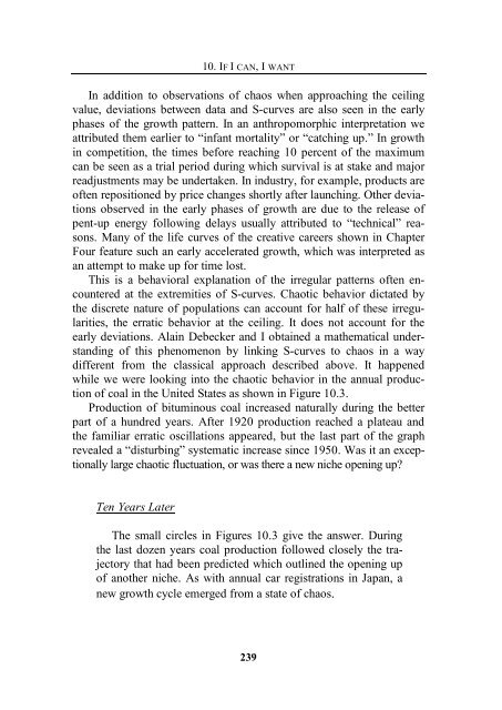
- Page 239: 10. IF I CAN, I WANT First commerci
- Page 243 and 244: 10. IF I CAN, I WANT Between two su
- Page 245 and 246: 10. IF I CAN, I WANT The state depi
- Page 247: 10. IF I CAN, I WANT to sustain one
- Page 250 and 251: 11. FORECASTING DESTINY announced i
- Page 252 and 253: 11. FORECASTING DESTINY The “natu
- Page 254 and 255: 11. FORECASTING DESTINY In 1975, as
- Page 256 and 257: 11. FORECASTING DESTINY The country
- Page 258 and 259: 11. FORECASTING DESTINY feedback me
- Page 260 and 261: 11. FORECASTING DESTINY States, rec
- Page 262 and 263: 11. FORECASTING DESTINY in 1991 pro
- Page 264 and 265: 11. FORECASTING DESTINY least four
- Page 266 and 267: 11. FORECASTING DESTINY United Stat
- Page 268 and 269: 11. FORECASTING DESTINY which would
- Page 271 and 272: EPILOGUE • • • We are in Cent
- Page 273 and 274: EPILOGUE Fads and media stories abo
- Page 275 and 276: APPENDICES 273
- Page 277 and 278: APPENDIX A The Predator-Prey Equati
- Page 279 and 280: APPENDIX A the two varieties will b
- Page 281 and 282: APPENDIX A By assigning weights to
- Page 283 and 284: APPENDIX B As an example, let us co
- Page 285 and 286: APPENDIX C Additional Figures THE N
- Page 287 and 288: APPENDIX C POPULATIONS OF CARS GROW
- Page 289 and 290: APPENDIX C RAILWAY NETWORKS GROW LI
- Page 291 and 292:
APPENDIX C GOTHIC CATHEDRALS APPEND
- Page 293 and 294:
APPENDIX C OIL PRODUCTION AND DISCO
- Page 295 and 296:
APPENDIX C ERNEST HEMINGWAY (1899-1
- Page 297 and 298:
APPENDIX C THE BIRTH RATE OF AMERIC
- Page 299 and 300:
APPENDIX C 296
- Page 301 and 302:
APPENDIX C WORLD WAR II FAVORED TUB
- Page 303 and 304:
APPENDIX C THE EXIT OF STEAM ENGINE
- Page 305 and 306:
APPENDIX C 302
- Page 307 and 308:
APPENDIX C THE DESTRUCTION OF THRES
- Page 309 and 310:
APPENDIX C WARS MAY INTERFERE WITH
- Page 311 and 312:
APPENDIX C COMPETITION BETWEEN TRAN
- Page 313 and 314:
APPENDIX C ANNUAL ENERGY CONSUMPTIO
- Page 315 and 316:
APPENDIX C THE GROWTH OF AIR TRAFFI
- Page 317 and 318:
APPENDIX C Annual registrations 6,0
- Page 319 and 320:
APPENDIX C POPULARIZED DEATHS HAVE
- Page 322 and 323:
NOTES AND SOURCES Prologue 1. Donel
- Page 324 and 325:
NOTES AND SOURCES the Law Followed
- Page 326 and 327:
NOTES AND SOURCES 4. For examples s
- Page 328 and 329:
NOTES AND SOURCES bile Road to Tech
- Page 330 and 331:
NOTES AND SOURCES 2. For a brief de
- Page 332:
NOTES AND SOURCES Appendix B: Expec
- Page 335 and 336:
ACKNOWLEDGEMENTS Bagwell, my initia