Applicazioni della teoria del minimax a problemi ... - Portale Posta DMI

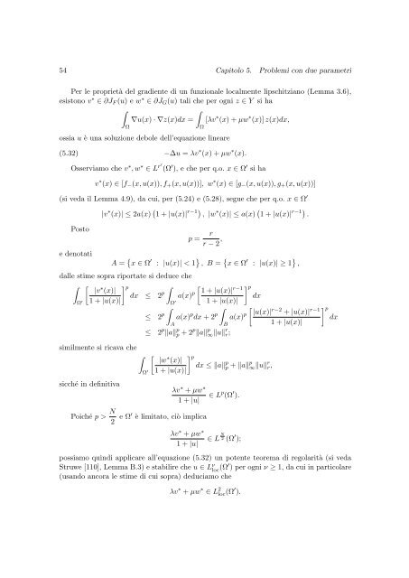
54 Capitolo 5. Problemi con due parametri
Per le proprietà del gradiente di un funzionale localmente lipschitziano (Lemma 3.6),
esistono v ∗ ∈ ∂JF (u) e w ∗ ∈ ∂JG(u) tali che per ogni z ∈ Y si ha
Ω
∇u(x) · ∇z(x)dx =
ossia u è una soluzione debole dell’equazione lineare
[λv
Ω
∗ (x) + µw ∗ (x)] z(x)dx,
(5.32) −∆u = λv ∗ (x) + µw ∗ (x).
Osserviamo che v∗ , w∗ ∈ Lr′ (Ω ′ ), e che per q.o. x ∈ Ω ′ si ha
v ∗ (x) ∈ [f−(x, u(x)), f+(x, u(x))], w ∗ (x) ∈ [g−(x, u(x)), g+(x, u(x))]
(si veda il Lemma 4.9), da cui, per (5.24) e (5.28), segue che per q.o. x ∈ Ω ′
Posto
e denotati
|v ∗ (x)| ≤ 2a(x) 1 + |u(x)| r−1 , |w ∗ (x)| ≤ a(x) 1 + |u(x)| r−1 .
A = x ∈ Ω ′
p = r
r − 2 ,
: |u(x)| < 1 , B = x ∈ Ω ′
: |u(x)| ≥ 1 ,
dalle stime sopra riportate si deduce che
Ω ′
|v∗ p
(x)|
dx
1 + |u(x)|
≤ 2 p
Ω ′
a(x) p
≤
1 + |u(x)| r−1 p
dx
1 + |u(x)|
2 p
a(x)
A
p dx + 2 p
a(x)
B
p
|u(x)| r−2 + |u(x)| r−1 p
dx
1 + |u(x)|
≤ 2 p a p p + 2 p a p ∞u r r;
similmente si ricava che
sicché in definitiva
Ω ′
|w∗ p
(x)|
dx ≤ a
1 + |u(x)|
p p + a p ∞u r r,
λv ∗ + µw ∗
1 + |u| ∈ Lp (Ω ′ ).
Poiché p > N
2 e Ω′ è limitato, ciò implica
λv ∗ + µw ∗
1 + |u|
∈ L N
2 (Ω ′ );
possiamo quindi applicare all’equazione (5.32) un potente teorema di regolarità (si veda
Struwe [110], Lemma B.3) e stabilire che u ∈ L ν loc (Ω′ ) per ogni ν ≥ 1, da cui in particolare
(usando ancora le stime di cui sopra) deduciamo che
λv ∗ + µw ∗ ∈ L 2 loc (Ω′ ).