xxiii πανελληνιο ÏƒÏ Î½ÎµÎ´ÏÎ¹Î¿ Ï†Ï ÏƒÎ¹ÎºÎ·Ï‚ στερεας καταστασης & επιστημης ...

A low-T study of the 3d random-field Ising model: The critical disorder strength
N.G. Fytas 1* and A. Malakis 1
1 University of Athens, Physics Department, Section of Solid State Physics, Panepistimiopolis, GR 157 84 Athens
*nfytas@phys.uoa.gr
The random-field Ising model (RFIM) [1] has been extensively studied [2] both because of its interest as a ‘simple’ frustrated
system and because of its relevance to experiments, especially those on the diluted antiferromagnet in a uniform field [2].
The Hamiltonian describing the model is
1.0
H =−J∑ SiSj −∑ hS
i i
, where S i
are Ising
< i,
j>
i
h RF
=2.1 (from h RF
=2.25)
L=8
h
spins, J > 0 is the nearest-neighbors
RF
=2.1 (WL)
0.8 h RF
=2.2(from h RF
=2.25)
ferromagnetic interaction, and h
i
are
h RF
=2.2 (WL)
independent quenched random-fields obtained
h from a bimodal distribution of the form:
0.6
RF
=2.25 (WL)
h RF
=2.3 (from h RF
=2.25)
1
Ph (
i) = [ δ( hi − hRF) + δ( hi + hRF)
]. h
RF
is the
h RF
=2.3 (WL)
2
0.4
0.2
h RF
=2.4 (from h RF
=2.25)
h RF
=2.4 (WL)
disorder strength, also called randomness of the
system. Although the critical behavior of the
model is not fully clarified, it has been proved
that an ordered phase exists for sufficiently low
temperature and disorder strength, and
dimension d > 2 [1]. At low values of the
C
disorder strength and temperature, the system is
in a ferromagnetic phase, and at high
temperatures or disorder strength, the system is
paramagnetic. The phase boundary of the model
is bounded at zero temperature from the critical
value of the disorder strength, denoted as h c RF
,
above which no phase transition occurs. This
critical strength value for the Gaussian RFIM is
known to be of the order of 2.30(5) (see Refs. [3,4] and references therein), while for the bimodal RFIM our recent high-T
study, using strength values h
RF
= 0.5,1,1.5 ,
c
3
and 2 , yielded h
RF
= 2.42(18) [5].
Here, we follow a low-T route, using data in
the neighborhood of the critical strength value.
We simulate the system at a randomness value
close to the expected critical, i.e. h
RF
= 2.25 .
2
L=4: h * =2.88(1)
Following our previous practice [6], we restrict
RF
L=8: h * =2.65(2)
the simulation in the dominant energy
RF
subspace. Since we are interested in an accurate
L=12: h * =2.56(3)
RF extrapolation also for values h
RF
> 2.25 , we
L=16: h *
1
=2.51(4)
RF use only a restriction for the right-end of the
L=20: h * =2.48(6)
RF
dominant energy subspace, including all the
low-energy spectrum down to the ground state.
We implement the Wang-Landau (WL)
algorithm [7] in order to obtain the density of
states (DOS) GE ( ) and also accumulate at the
0
0 1 2 3 4 5 high levels of the WL process ( j
WL
= 16 − 20)
T
the double exchange-field energy histogram
h RF
0.0
0.5 1.0 1.5 2.0 2.5 3.0 3.5
T
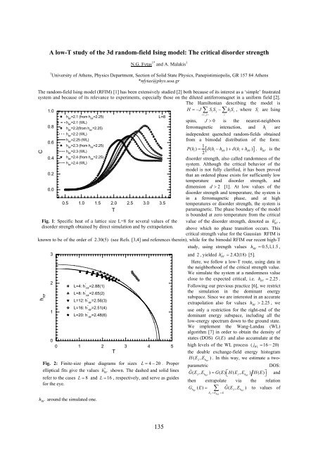
Fig. 1: Specific heat of a lattice size L=8 for several values of the
disorder strength obtained by direct simulation and by extrapolation.
Fig. 2: Finite-size phase diagrams for sizes L = 4 − 20 . Proper
elliptical fits give the values h * RF
shown. The dashed and solid lines
refer to the cases L = 8 and L = 16 , respectively, and serve as guides
for the eye.
h
RF
around the simulated one.
H( EJ, E
h RF
). In this way, we estimate a twoparametric
DOS:
GE (
J, Eh ) = GE ( ) ⎡ ( , )
RF ⎣
HEJ Eh
RF
HE ( ) ⎤
⎦
and
then extrapolate via the relation
G ( E) = ∑ G ( E , E ) to values of
hRF
J hRF
EJ
+ Eh RF
= E
135