xxiii πανελληνιο ÏƒÏ Î½ÎµÎ´ÏÎ¹Î¿ Ï†Ï ÏƒÎ¹ÎºÎ·Ï‚ στερεας καταστασης & επιστημης ...

Application of Thermal Quadrupoles Method for Modeling of AC impedance
in Thermoelectric Elements
D. Georgakaki * , E. Hatzikraniotis, J. Samaras, O. G. Ziogos, K. M. Paraskevopoulos
Solid State Section, Physics Department, Aristotle University, 54124 Thessaloniki, Greece
* dimge@physics.auth.gr
Introduction
The quadrupole method is an explicit method of the representation of heat transfer through multimaterials. It is based on
2x2 matrices that allow finding a linear relationship between the Laplace temperature and heat flux transformations at
boundaries (θ in , φ in ) and (θ out , φ out ) of the considered medium [1]. The multimaterial is thus considered as a thermal
transmission line, whose individual components contribute differently at the propagation of the thermal wave [2].
Using an AC electrical measurement, the frequency-domain response of a common thermoelectric element has been
obtained for various current loads. The effects of the thermal wave along the length of the measured sample were accurately
modeled using the quadrupole theory by taking into account the thermal impedances of the metal-semiconductor interfaces.
Experimental details
The sample is a single N-type Bi 2 Te 3 block of thickness d=2.5mm and cross section S=4mm. Two copper electrodes are
soldered to the sample ends and two copper wires connected to the electrodes supply the current (1mA AC+100mA DC) in a
10 -3 up to 10 2 Hz frequency range. The magnitude of the electrical impedance of the sample |Z|=V 0 /I 0 is measured by an
impedance meter (IM6) connected to the wires.
Thermal Quadrupole Modeling
Considering the one-dimensional heat transfer problem (x-direction) through a body of thickness d, the following
equations that relate the temperature and flux at x=0 with those at x=d are extracted [3]:
sinh( β ⋅ d)
θin
= cosh( β ⋅ d)
θout
+ φout
λSβ
(1)
φin
= λSβ
⋅sinh(
β ⋅ d)
θout
+ cosh( β ⋅ d)
φout
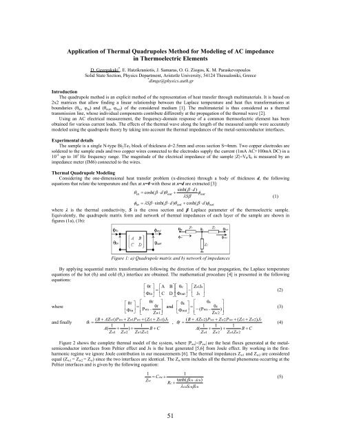
where λ is the thermal conductivity, S is the cross section and β Laplace parameter of the thermoelectric sample.
Equivalently, the quadrupole matrix form and network of thermal impedances of each layer of the sample are shown in
figures (1a), (1b):
Figure 1: a) Quadrupole matrix and b) network of impedances
By applying sequential matrix transformations following the direction of the heat propagation, the Laplace temperature
equations of the hot (θ f ) and cold (θ c ) interface are obtained. The mathematical procedure [4] is presented in the following
equations:
⎡ θf
⎤ ⎡A
B⎤⎡
θc
⎤ ⎡Zs1J
s⎤
⎢ ⎥ = ⎢ ⎥⎢
⎥ − ⎢ ⎥
(2)
⎣Φin⎦
⎣C
D⎦⎣Φout⎦
⎣ Js
⎦
where
and finally
⎡ θf
⎤ ⎡ θf
⎤
⎢ ⎥ = ⎢ θf
⎥ and
⎣Φin⎦
⎢Pws
−
⎣ Z
⎥
w1⎦
( B + AZw1)
Pws
+ Zw1Pws
+ ( Zs1
+ Zw1)
Js
θ c =
,
1 1 1
A(
+ ) + B + C
Zw1
Zw2
Zw1Zw
2
⎡ θc
⎤ ⎡ θc
⎤
⎢ ⎥ = ⎢ θc
⎥
(3)
⎢−
⎣Φout
(Pws
− )
⎦ ⎣ Z
⎥
w2 ⎦
( B + AZw2)
Pws
+ Zw2Pws
+ ( Zs1
+ Zw2)
Js
θ f =
(4)
1 1 1
A(
+ ) + B + C
Zw1
Zw2
Zw1Zw
2
Figure 2 shows the complete thermal model of the system, where |P ws |=|P sw | are the heat fluxes generated at the metalsemiconductor
interfaces from Peltier effect and Js is the heat generated [5,6] from Joule effect. By working in the firstharmonic
regime we ignore Joule contribution in our measurements [6]. The thermal impedances Z w1 and Z w2 are considered
equal (Z w1 = Z w2 = Z w ) since the two interfaces are identical. The Z w term includes all the thermal phenomena occurring at the
Peltier interfaces and is given by the following equation:
1
1
= Ccu
+
(5)
Zw
tanh(β cu ⋅ dcu)
Rc
+
λcuScuβcu
51