Perspektiv på välfärden 2004 (pdf) - Statistiska centralbyrån
Perspektiv på välfärden 2004 (pdf) - Statistiska centralbyrån
Perspektiv på välfärden 2004 (pdf) - Statistiska centralbyrån

Create successful ePaper yourself
Turn your PDF publications into a flip-book with our unique Google optimized e-Paper software.
Youth<br />
tion that change is a linear function of time. However,<br />
in this particular case the linear assumption<br />
is not realistic. For example, the typical pattern of<br />
income development is not linear continuous<br />
growth. What we observe is rather a curve-linear<br />
development signified by a rapid increase during<br />
the period a person establishes herself on the labour<br />
market, followed by a slower increase as she<br />
gets older, and eventually a decrease by the end of<br />
the life course. The income slope has therefore<br />
been specified with a relation of 0 with the t 0<br />
measure, 2 with th0e t 1 measure, and 3 with the t 2<br />
measure, expressing a curve-linear rather than a<br />
linear function of time. A linear function has been<br />
applied for the measurement of deprivation slope.<br />
The means of the manifest variables are constrained<br />
to zero. This, along with the fixed relations<br />
between the latent variables and the manifest<br />
variables, allows the latent variables to function as<br />
a ‘container’ of parameters of the random coefficients<br />
model. Thus, for the Intercept latent variable,<br />
a mean and a variance are estimated, where<br />
the variance represents individual differences in<br />
the intercept of the growth model. For the Slope<br />
variable as well, a mean and a variance are estimated,<br />
and here the variance parameter represents<br />
individual differences in linear change over time.<br />
Thus, the SEM ap0proach allows straightforward<br />
specification, estimation and interpretation of the<br />
growth models.<br />
Results<br />
In order to arrive at a model that is as parsimonious<br />
as possible, the following approach has been<br />
applied. The starting point is taken in a ‘full<br />
model’ estimating all relationships that follow<br />
from the analytic model in Figure 1. That is, the<br />
variables in the first block affect all the others,<br />
variables in block two are correlated and the variables<br />
in block three are affected by all previous<br />
variables at the same time as they are interrelated,<br />
as shown in the figure. Insignificant estimates (tvalue<br />
less than 1.96) have thereafter been lifted<br />
from the model one by one in order to find a parsimonious<br />
model that fits the data at least as well<br />
as the full model. The strategy resembles what<br />
Jöreskog (1993) called ‘model generating,’ and as<br />
a result only significant estimates are displayed in<br />
the tables 4 . The model has been specified in<br />
4 In addition to those displayed are the correlations<br />
between sets of dummy variables estimated, that is<br />
dummies for class of origin, education and unemployment.<br />
This is necessary to get an acceptable fit of the<br />
model, but reflects nothing more than the obvious fact<br />
that they are mutually exclusive. For the exogenous<br />
class dummies, it is the observed variables that are<br />
allowed to co-vary, while for the endogenous educa-<br />
74<br />
STREAMS 2.5, and estimated with AMOS 4. The<br />
results are displayed in two different tables.<br />
Manifest variables<br />
Table 4 shows parameters for the relationship<br />
between the exogenous variables age, gender and<br />
class of origin, and the set of endogenous variables<br />
that indicate the youth situation. Thus, the<br />
table relates to manifest variables in the two first<br />
blocks of the analytical model (Figure 1).<br />
In table 4 we can see that the older the population<br />
becomes, the more likely it is that they have<br />
attained a longer education, are employed, have<br />
left the nest, and have a child of their own. Hence,<br />
the pattern revealed is more or less what can be<br />
expected when analysing a population that is presumably<br />
in a transitional phase into adulthood.<br />
The next variable, gender, is more interesting, as<br />
it reveals substantial differences between women<br />
and men. Both short- and long-term unemployment<br />
are more common among women. This is<br />
also true for social assistance, although it must be<br />
kept in mind that this variable is somewhat problematic<br />
due to underreporting (see footnote 3). As<br />
expected, women also leave the nest earlier than<br />
do men, and they are also more likely to become a<br />
parent at a young age.<br />
The estimates related to class of origin should<br />
be interpreted as contrasts to the reference group,<br />
which in this case consists of blue-collar workers.<br />
It is apparent that those with middle and higher<br />
white-collar worker class of origin deviate from<br />
the rest. H0ere we find a higher incidence of<br />
higher education, a larger share of students, especially<br />
among the older sections of the population,<br />
which is shown by the impact on the interaction<br />
between being a student and age (older students,<br />
who are usually those involved in tertiary education,<br />
more often come from white-collar homes).<br />
As a natural consequence, being unemployed is<br />
less likely if the class of origin is middle or higher<br />
white-collar worker. It is also less common that<br />
people with a white-collar background have children<br />
of their own at a young age. Thus, table<br />
4confirms a picture that we, on the basis of earlier<br />
research, more or less expected. The reproduction<br />
of a class society shines through the results of the<br />
analysis and there is also a gendered pattern<br />
showing that0 young women seem to become<br />
what is commonly defined as "adults" earlier,<br />
because of their earlier nest leaving and higher<br />
likelihood of becoming a parent at an early age. In<br />
addition to the regression estimates (specified as<br />
causal relations), correlations are also estimated<br />
between the variables relating to block two of<br />
Figure 1. The significant results are shown in<br />
tion and unemployment dummies, it is the error term<br />
that co-varies.