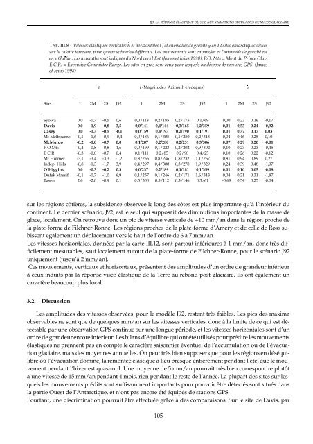
_hTAB. III.8 - Vitesses élastiques vertica<strong>le</strong>s_het horizonta<strong>le</strong>s_l, et anomalies de gravité_gen 12 sites antarctiques situéssur la calotte terrestre, pour quatre scénarios différents. Les mouvements sont en mm/an et l’anomalie de gravité estenGal/an. Les azimuths sont indiqués du Nord vers l’Est (James et Ivins 1998). P.O. Mts = Mont du Prince Olav,E.C.R. = Executive Committee Range. Les sites en gras sont ceux pour <strong>le</strong>squels on dispose de mesures GPS. (Jameset Ivins 1998)_l(Magnitude/Site 1 2M 2S J92 1 2M 2S J92 1 2M 2S J92_gx3. LA RÉPONSE ÉLASTIQUE DU SOL AUX VARIATIONS SÉCULAIRES DE MASSE GLACIAIRE.Azimuth en degres)Syowa 0,0 -0,7 -0,5 0,6 0,0/118 0,2/185 0,2/175 0,1/69 0,00 0,23 0,16 -0,17Davis 0,0 -1,9 -0,8 3,5 0,0/141 0,4/144 0,3/165 1,2/359 0,01 0,53 0,24 -0,92Casey 0,0 -1,3 -0,5 -0,1 0,0/159 0,4/193 0,2/190 0,1/191 0,01 0,37 0,17 0,03Mt Melbourne -0,1 -1,6 -0,9 -0,4 0,0/186 0,1/305 0,1/250 0,2/315 0,04 0,46 0,25 0,10McMurdo -0,2 -1,0 -0,7 0,0 0,1/207 0,2/280 0,2/231 0,3/306 0,07 0,29 0,20 -0,01P O Mts -0,4 -0,8 -0,8 1,6 0,0/199 0,1/223 0,2/202 0,9/302 0,10 0,23 0,23 -0,45E C R -0,3 -0,8 -0,7 0,4 0,1/111 0,2/85 0,2/98 0,4/25 0,10 0,26 0,22 -0,12Mt Hulmer -3,1 -3,4 -3,3 -1,2 0,8/255 0,8/246 0,8/232 1,1/267 0,81 0,94 0,89 0,27Indep. Hills -0,8 -1,3 -1,7 3,9 0,4/297 0,4/300 0,3/278 1,9/329 0,24 0,39 0,48 -1,07O’Higgins 0,0 -0,3 -0,2 0,3 0,0/237 0,2/189 0,1/181 0,1/359 0,01 0,10 0,05 -0,08Dufek Massif -0,1 -0,7 -1,0 6,9 0,1/257 0,1/246 0,2/171 1,6/343 0,04 0,21 0,31 -1,87Basen 2,6 -2,0 -0,9 0,1 0,5/300 0,5/112 0,3/146 0,3/61 -0,68 0,54 0,25 -0,04sur <strong>le</strong>s régions côtières, la subsidence observée <strong>le</strong> long des côtes est plus importante qu’à l’intérieur ducontinent. Le dernier scénario, J92, est <strong>le</strong> seul qui supposait des diminutions importantes de la masse deglace, loca<strong>le</strong>ment. On retrouve donc un pic de vitesse vertica<strong>le</strong> de +10 mm/an dans la région proche dela plate-forme de Filchner-Ronne. Les régions proches de la plate-forme d’Amery et de cel<strong>le</strong> de Ross subissentéga<strong>le</strong>ment un déplacement vers <strong>le</strong> haut de l’ordre de 6 à 7 mm/an.Les vitesses horizonta<strong>le</strong>s, données par la carte III.12, sont partout inférieures à 1 mm/an, donc très diffici<strong>le</strong>mentmesurab<strong>le</strong>s, sauf loca<strong>le</strong>ment autour de la plate-forme de Filchner-Ronne, pour <strong>le</strong> scénario J92uniquement (jusqu’à 2 mm/an).Ces mouvements, verticaux et horizontaux, présentent des amplitudes d’un ordre de grandeur inférieurà ceux induits par la réponse visco-élastique de la Terre au rebond post-glaciaire. Ils ont éga<strong>le</strong>ment uncaractère beaucoup plus local.3.2. DiscussionLes amplitudes des vitesses observées, pour <strong>le</strong> modè<strong>le</strong> J92, restent très faib<strong>le</strong>s. Les pics des maximaobservab<strong>le</strong>s ne sont que de quelques mm/an sur <strong>le</strong>s vitesses vertica<strong>le</strong>s, donc à la limite de ce qui est détectab<strong>le</strong>par une observation GPS continue sur une longue période, et <strong>le</strong>s vitesses horizonta<strong>le</strong>s sont d’unordre de grandeur encore inférieur. Les bilans d’équilibre qui ont été utilisés pour prédire <strong>le</strong>s mouvementsélastiques ne prennent pas en compte <strong>le</strong> caractère saisonnier éventuel de l’accumulation ou de l’évacuationglaciaire, mais des moyennes annuel<strong>le</strong>s. On peut très bien supposer que pour <strong>le</strong>s régions en déséquilibreoù l’évacuation domine, la remontée élastique a lieu presque entièrement pendant l’été, que <strong>le</strong> mouvementpendant l’hiver est quasi-nul. Une moyenne de 5 mm/an pourrait très bien correspondre plutôtà une vitesse de 15 mm/an pendant 4 mois, rien pendant <strong>le</strong> reste de l’année. La plupart des sites sur <strong>le</strong>squels<strong>le</strong>s mouvements prédits sont suffisamment importants pour pouvoir être détectés sont situés dansla partie Ouest de l’Antarctique, et n’ont pas encore été équipés de stations GPS.Pourtant, une discrimination pourrait être effectuée grâce à des comparaisons. Sur <strong>le</strong> site de Davis, par105
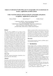
CHAPITRE III. COMPORTEMENT ACTUEL DE LA CALOTTE GLACIAIRE ANTARCTIQUE.FIG. III.12 - Vitesses horizonta<strong>le</strong>s de la croûte résultant de l’application des quatre scénarios décrits plus haut.L’échel<strong>le</strong> est indiquée au centre (James et Ivins 1998).exemp<strong>le</strong>, qui présente l’avantage d’être situé au voisinage de la plate-forme d’Amery, la différence devitesse vertica<strong>le</strong> entre <strong>le</strong> modè<strong>le</strong> J92 (<strong>le</strong> seul à tenir compte de décharges glaciaires loca<strong>le</strong>s importantes)et l’autre extrême, <strong>le</strong>(scénario 2 massique))qui concentre l’accumulation sur <strong>le</strong>s côtes, est de plus de 5mm/an. Une mesure sur plusieurs années a donc un bon pouvoir discriminant, d’autant que l’une desvitesses vertica<strong>le</strong>s prédites correspond à une subsidence et l’autre à un soulèvement. Les amplitudes desmouvements horizontaux sur ce même site de Davis restent très faib<strong>le</strong>s, mais au moins <strong>le</strong>urs directionssont-el<strong>le</strong>s radica<strong>le</strong>ment différentes : 144oEst pour <strong>le</strong>(scénario 2 massique), 359opour <strong>le</strong> scénario J92. Ladifférence entre <strong>le</strong>s anomalies de gravité est éga<strong>le</strong>ment significative, puisque l’anomalie résultant de l’applicationdu(scénario 2 massique)est de 0,53Gal/an, cel<strong>le</strong> de J92 de -0,92Gal/an.106
- Page 1 and 2:
ThesedeDoctoratdel'ObservatoiredePa
- Page 3 and 4:
Remerciements.La fin de cette thès
- Page 6 and 7:
Table des matièresIntroduction gé
- Page 8 and 9:
3.1. Résultats des modèles. . . .
- Page 10 and 11:
2. Réponse de la Terre à une char
- Page 12 and 13:
GPS Global Positioning System.HOB2
- Page 14 and 15:
INTRODUCTIONINTRODUCTION GÉNÉRALE
- Page 16:
INTRODUCTIONments sur la stabilité
- Page 20 and 21:
CHAPITRE IDONNÉES GÉNÉRALES SUR
- Page 22 and 23:
x1. LA GÉOGRAPHIE DE L’ANTARCTIQ
- Page 24 and 25:
x1. LA GÉOGRAPHIE DE L’ANTARCTIQ
- Page 26 and 27:
x1. LA GÉOGRAPHIE DE L’ANTARCTIQ
- Page 28 and 29:
x3. GÉOLOGIE ET GÉOPHYSIQUE.balay
- Page 30 and 31:
x3. GÉOLOGIE ET GÉOPHYSIQUE.- Sur
- Page 32 and 33:
x4. LA DÉCOUVERTE DE L’ANTARCTIQ
- Page 34 and 35:
x4. LA DÉCOUVERTE DE L’ANTARCTIQ
- Page 36 and 37:
x4. LA DÉCOUVERTE DE L’ANTARCTIQ
- Page 38 and 39:
CHAPITRE IIL’ISOSTASIE APPLIQUÉE
- Page 40 and 41:
x1. L’ISOSTASIE TERRESTRE ET SON
- Page 42 and 43:
affectés par la réponse terrestre
- Page 44 and 45:
x1. L’ISOSTASIE TERRESTRE ET SON
- Page 46 and 47:
x1. L’ISOSTASIE TERRESTRE ET SON
- Page 48 and 49:
x2. MODÈLES DE DÉGLACIATION ET CA
- Page 50 and 51:
x2. MODÈLES DE DÉGLACIATION ET CA
- Page 52 and 53:
x2. MODÈLES DE DÉGLACIATION ET CA
- Page 54 and 55:
x2. MODÈLES DE DÉGLACIATION ET CA
- Page 56 and 57: x2. MODÈLES DE DÉGLACIATION ET CA
- Page 58 and 59: x2. MODÈLES DE DÉGLACIATION ET CA
- Page 60 and 61: x2. MODÈLES DE DÉGLACIATION ET CA
- Page 62 and 63: x2. MODÈLES DE DÉGLACIATION ET CA
- Page 64 and 65: x2. MODÈLES DE DÉGLACIATION ET CA
- Page 66 and 67: x2. MODÈLES DE DÉGLACIATION ET CA
- Page 68 and 69: x3. LE CAS PARTICULIER DE L’ANTAR
- Page 70 and 71: x3. LE CAS PARTICULIER DE L’ANTAR
- Page 72 and 73: x3. LE CAS PARTICULIER DE L’ANTAR
- Page 74 and 75: x3. LE CAS PARTICULIER DE L’ANTAR
- Page 76 and 77: x3. LE CAS PARTICULIER DE L’ANTAR
- Page 78 and 79: x3. LE CAS PARTICULIER DE L’ANTAR
- Page 80 and 81: x3. LE CAS PARTICULIER DE L’ANTAR
- Page 82 and 83: x3. LE CAS PARTICULIER DE L’ANTAR
- Page 84 and 85: x4. CONCLUSION.4. Conclusion.On a p
- Page 86 and 87: CHAPITRE IIICOMPORTEMENT ACTUEL DE
- Page 88 and 89: x1. LES TENDANCES ACTUELLES DE L’
- Page 90 and 91: x1. LES TENDANCES ACTUELLES DE L’
- Page 92 and 93: x1. LES TENDANCES ACTUELLES DE L’
- Page 94 and 95: x1. LES TENDANCES ACTUELLES DE L’
- Page 96 and 97: x1. LES TENDANCES ACTUELLES DE L’
- Page 98 and 99: x2. BILAN ACTUEL DE L’ÉQUILIBRE
- Page 100 and 101: _x2. BILAN ACTUEL DE L’ÉQUILIBRE
- Page 102 and 103: x2. BILAN ACTUEL DE L’ÉQUILIBRE
- Page 104 and 105: x3. LA RÉPONSE ÉLASTIQUE DU SOL A
- Page 108 and 109: x4. UNE ALTERNATIVE : LES MODÈLES
- Page 110 and 111: x4. UNE ALTERNATIVE : LES MODÈLES
- Page 112 and 113: x4. UNE ALTERNATIVE : LES MODÈLES
- Page 114 and 115: x4. UNE ALTERNATIVE : LES MODÈLES
- Page 116 and 117: d dt=du dt6;5d(gm)Ordx4. UNE ALTERN
- Page 118: x5. CONCLUSION.ley estime que la te
- Page 121 and 122: CHAPITRE IV. MOUVEMENTS NE PROVENAN
- Page 123 and 124: CHAPITRE IV. MOUVEMENTS NE PROVENAN
- Page 125 and 126: CHAPITRE IV. MOUVEMENTS NE PROVENAN
- Page 127 and 128: CHAPITRE IV. MOUVEMENTS NE PROVENAN
- Page 130 and 131: CHAPITRE ISPÉCIFICITÉS DU TRAITEM
- Page 132 and 133: x1. GÉOMÉTRIE DU RÉSEAU.du trait
- Page 134 and 135: x2. LES ORBITES DES SATELLITES GPS
- Page 136 and 137: x2. LES ORBITES DES SATELLITES GPS
- Page 138 and 139: x2. LES ORBITES DES SATELLITES GPS
- Page 140 and 141: x3. ACTIVITÉ IONOSPHÉRIQUE.quanti
- Page 142 and 143: x3. ACTIVITÉ IONOSPHÉRIQUE.TAB. I
- Page 144 and 145: x4. L’EFFET DE LA NEIGE SUR LE GP
- Page 146 and 147: x4. L’EFFET DE LA NEIGE SUR LE GP
- Page 148 and 149: x5. CONCLUSION.5. Conclusion.Traite
- Page 150 and 151: CHAPITRE IILE TRAITEMENT DES DONNÉ
- Page 152 and 153: x1. DONNÉES GPS DISPONIBLES.0˚330
- Page 154 and 155: x1. DONNÉES GPS DISPONIBLES.DUM1MA
- Page 156 and 157:
x2. CALCUL SUR LES STATIONS IGS ANT
- Page 158 and 159:
x2. CALCUL SUR LES STATIONS IGS ANT
- Page 160 and 161:
x2. CALCUL SUR LES STATIONS IGS ANT
- Page 162 and 163:
x2. CALCUL SUR LES STATIONS IGS ANT
- Page 164 and 165:
x2. CALCUL SUR LES STATIONS IGS ANT
- Page 166 and 167:
x2. CALCUL SUR LES STATIONS IGS ANT
- Page 168 and 169:
x2. CALCUL SUR LES STATIONS IGS ANT
- Page 170 and 171:
x3. CALCUL EN RÉSEAU ÉLARGI.3. Ca
- Page 172 and 173:
x3. CALCUL EN RÉSEAU ÉLARGI.exist
- Page 174 and 175:
x3. CALCUL EN RÉSEAU ÉLARGI.TAB.
- Page 176 and 177:
x3. CALCUL EN RÉSEAU ÉLARGI.5040N
- Page 178 and 179:
x3. CALCUL EN RÉSEAU ÉLARGI.97, a
- Page 180 and 181:
x3. CALCUL EN RÉSEAU ÉLARGI.Latit
- Page 182 and 183:
x3. CALCUL EN RÉSEAU ÉLARGI.Casey
- Page 184:
x4. CONCLUSION.particulièrement im
- Page 187 and 188:
CHAPITRE III. ANALYSE GÉODÉSIQUE
- Page 189 and 190:
CHAPITRE III. ANALYSE GÉODÉSIQUE
- Page 191 and 192:
CHAPITRE III. ANALYSE GÉODÉSIQUE
- Page 193 and 194:
CHAPITRE III. ANALYSE GÉODÉSIQUE
- Page 195 and 196:
CHAPITRE III. ANALYSE GÉODÉSIQUE
- Page 197 and 198:
CHAPITRE III. ANALYSE GÉODÉSIQUE
- Page 199 and 200:
CHAPITRE III. ANALYSE GÉODÉSIQUE
- Page 201 and 202:
CHAPITRE III. ANALYSE GÉODÉSIQUE
- Page 203 and 204:
CHAPITRE III. ANALYSE GÉODÉSIQUE
- Page 205 and 206:
CHAPITRE III. ANALYSE GÉODÉSIQUE
- Page 207 and 208:
CHAPITRE III. ANALYSE GÉODÉSIQUE
- Page 209 and 210:
CHAPITRE III. ANALYSE GÉODÉSIQUE
- Page 211 and 212:
CHAPITRE III. ANALYSE GÉODÉSIQUE
- Page 213 and 214:
CHAPITRE III. ANALYSE GÉODÉSIQUE
- Page 215 and 216:
CHAPITRE III. ANALYSE GÉODÉSIQUE
- Page 217 and 218:
CHAPITRE III. ANALYSE GÉODÉSIQUE
- Page 219 and 220:
CHAPITRE III. ANALYSE GÉODÉSIQUE
- Page 221 and 222:
CHAPITRE III. ANALYSE GÉODÉSIQUE
- Page 223 and 224:
CHAPITRE III. ANALYSE GÉODÉSIQUE
- Page 225 and 226:
CHAPITRE IV. INTERPRÉTATION GÉOPH
- Page 227 and 228:
CHAPITRE IV. INTERPRÉTATION GÉOPH
- Page 229 and 230:
CHAPITRE IV. INTERPRÉTATION GÉOPH
- Page 231 and 232:
CHAPITRE IV. INTERPRÉTATION GÉOPH
- Page 233 and 234:
CHAPITRE IV. INTERPRÉTATION GÉOPH
- Page 235 and 236:
CHAPITRE IV. INTERPRÉTATION GÉOPH
- Page 237 and 238:
CHAPITRE IV. INTERPRÉTATION GÉOPH
- Page 239 and 240:
CHAPITRE IV. INTERPRÉTATION GÉOPH
- Page 241 and 242:
CHAPITRE IV. INTERPRÉTATION GÉOPH
- Page 243 and 244:
CHAPITRE IV. INTERPRÉTATION GÉOPH
- Page 245 and 246:
CHAPITRE IV. INTERPRÉTATION GÉOPH
- Page 247 and 248:
CHAPITRE IV. INTERPRÉTATION GÉOPH
- Page 249 and 250:
CHAPITRE IV. INTERPRÉTATION GÉOPH
- Page 251 and 252:
CHAPITRE IV. INTERPRÉTATION GÉOPH
- Page 253 and 254:
CHAPITRE IV. INTERPRÉTATION GÉOPH
- Page 255 and 256:
CHAPITRE IV. INTERPRÉTATION GÉOPH
- Page 257 and 258:
CHAPITRE IV. INTERPRÉTATION GÉOPH
- Page 259 and 260:
CHAPITRE IV. INTERPRÉTATION GÉOPH
- Page 261 and 262:
CHAPITRE IV. INTERPRÉTATION GÉOPH
- Page 263 and 264:
CHAPITRE IV. INTERPRÉTATION GÉOPH
- Page 265 and 266:
CHAPITRE IV. INTERPRÉTATION GÉOPH
- Page 268 and 269:
CONCLUSIONCONCLUSION GÉNÉRALE.Cro
- Page 270 and 271:
CONCLUSIONlongues devraient permett
- Page 272 and 273:
RÉFÉRENCESRéférencesAGNEW, D. C
- Page 274 and 275:
RÉFÉRENCESBUDD, W. F. et I. N. SM
- Page 276 and 277:
RÉFÉRENCESHUGHES, T. J., G. H. DE
- Page 278 and 279:
RÉFÉRENCESLANGBEIN, J. et H. JOHN
- Page 280 and 281:
RÉFÉRENCESOERLEMANS, J. Model exp
- Page 282 and 283:
RÉFÉRENCESSKVARCA, P. Changes and
- Page 284:
RÉFÉRENCESWYATT, F. K. Measuremen
- Page 287 and 288:
parW(;Le formalisme spectral se fon
- Page 289 and 290:
L(0; 0;t0)=X`;mL`m(t0)Y`m(0;ANNEXE
- Page 291 and 292:
(; termen(; ;t)=N`m Xn=1n(; ;t)ANNE
- Page 293 and 294:
oùIICE L`m(t)=wSEO Lǹm=wSn;EO `m(
- Page 295 and 296:
ANNEXE A. CALCUL DE DÉFORMATIONS D
- Page 297 and 298:
ANNEXE B. QUELQUES RAPPELS THÉORIQ
- Page 299 and 300:
t0est le temps d’intégration, o
- Page 301 and 302:
em(t)=Zt =(f0+a)(tt0)+12b(tt0)2+em(
- Page 303 and 304:
Les termes principaux dans l’équ
- Page 305 and 306:
ANNEXE B. QUELQUES RAPPELS THÉORIQ
- Page 307 and 308:
:ai=sin(Elv)=hibi=cos2(Elv)=2ahi A2
- Page 309 and 310:
ANNEXE B. QUELQUES RAPPELS THÉORIQ
- Page 311 and 312:
ANNEXE C. SÉRIES TEMPORELLES ISSUE
- Page 313 and 314:
ANNEXE C. SÉRIES TEMPORELLES ISSUE
- Page 315 and 316:
ANNEXE C. SÉRIES TEMPORELLES ISSUE
- Page 317 and 318:
ANNEXE C. SÉRIES TEMPORELLES ISSUE
- Page 319 and 320:
ANNEXE C. SÉRIES TEMPORELLES ISSUE
- Page 321 and 322:
ANNEXE C. SÉRIES TEMPORELLES ISSUE
- Page 323 and 324:
ANNEXE C. SÉRIES TEMPORELLES ISSUE
- Page 325 and 326:
ANNEXE C. SÉRIES TEMPORELLES ISSUE
- Page 328 and 329:
ANNEXE DCAS PARTICULIER : MESURE PA
- Page 330:
Latitude en m.−21.00−22.00−23