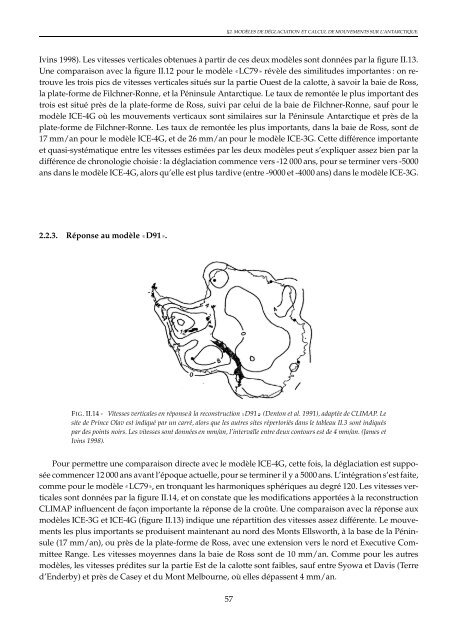
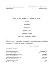
x2. MODÈLES DE DÉGLACIATION ET CALCUL DE MOUVEMENTS SUR L’ANTARCTIQUE.Ivins 1998). Les vitesses vertica<strong>le</strong>s obtenues à partir de ces deux modè<strong>le</strong>s sont données par la figure II.13.Une comparaison avec la figure II.12 pour <strong>le</strong> modè<strong>le</strong>(LC79)révè<strong>le</strong> des similitudes importantes : on retrouve<strong>le</strong>s trois pics de vitesses vertica<strong>le</strong>s situés sur la partie Ouest de la calotte, à savoir la baie de Ross,la plate-forme de Filchner-Ronne, et la Péninsu<strong>le</strong> Antarctique. Le taux de remontée <strong>le</strong> plus important destrois est situé près de la plate-forme de Ross, suivi par celui de la baie de Filchner-Ronne, sauf pour <strong>le</strong>modè<strong>le</strong> ICE-4G où <strong>le</strong>s mouvements verticaux sont similaires sur la Péninsu<strong>le</strong> Antarctique et près de laplate-forme de Filchner-Ronne. Les taux de remontée <strong>le</strong>s plus importants, dans la baie de Ross, sont de17 mm/an pour <strong>le</strong> modè<strong>le</strong> ICE-4G, et de 26 mm/an pour <strong>le</strong> modè<strong>le</strong> ICE-3G. Cette différence importanteet quasi-systématique entre <strong>le</strong>s vitesses estimées par <strong>le</strong>s deux modè<strong>le</strong>s peut s’expliquer assez bien par ladifférence de chronologie choisie : la déglaciation commence vers -12 000 ans, pour se terminer vers -5000ans dans <strong>le</strong> modè<strong>le</strong> ICE-4G, alors qu’el<strong>le</strong> est plus tardive (entre -9000 et -4000 ans) dans <strong>le</strong> modè<strong>le</strong> ICE-3G.2.2.3. Réponse au modè<strong>le</strong>((D91)).FIG. II.14 - Vitesses vertica<strong>le</strong>s en réponse à la reconstruction(D91)(Denton et al. 1991), adaptée de CLIMAP. Lesite de Prince Olav est indiqué par un carré, alors que <strong>le</strong>s autres sites répertoriés dans <strong>le</strong> tab<strong>le</strong>au II.3 sont indiquéspar des points noirs. Les vitesses sont données en mm/an, l’interval<strong>le</strong> entre deux contours est de 4 mm/an. (James etIvins 1998).Pour permettre une comparaison directe avec <strong>le</strong> modè<strong>le</strong> ICE-4G, cette fois, la déglaciation est supposéecommencer 12 000 ans avant l’époque actuel<strong>le</strong>, pour se terminer il y a 5000 ans. L’intégration s’est faite,comme pour <strong>le</strong> modè<strong>le</strong>((LC79), en tronquant <strong>le</strong>s harmoniques sphériques au degré 120. Les vitesses vertica<strong>le</strong>ssont données par la figure II.14, et on constate que <strong>le</strong>s modifications apportées à la reconstructionCLIMAP influencent de façon importante la réponse de la croûte. Une comparaison avec la réponse auxmodè<strong>le</strong>s ICE-3G et ICE-4G (figure II.13) indique une répartition des vitesses assez différente. Le mouvements<strong>le</strong>s plus importants se produisent maintenant au nord des Monts Ellsworth, à la base de la Péninsu<strong>le</strong>(17 mm/an), ou près de la plate-forme de Ross, avec une extension vers <strong>le</strong> nord et Executive CommitteeRange. Les vitesses moyennes dans la baie de Ross sont de 10 mm/an. Comme pour <strong>le</strong>s autresmodè<strong>le</strong>s, <strong>le</strong>s vitesses prédites sur la partie Est de la calotte sont faib<strong>le</strong>s, sauf entre Syowa et Davis (Terred’Enderby) et près de Casey et du Mont Melbourne, où el<strong>le</strong>s dépassent 4 mm/an.57
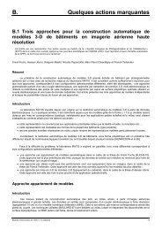
CHAPITRE II. ISOSTASIE EN ANTARCTIQUE. LA DERNIÈRE DÉGLACIATION ET SES CONSÉQUENCES.2.3. Discussion._h _gSite LC79 ICE-3G ICE-4G D91 LC79 ICE-3G D91Syowa 0,7 0,8 1,6 1,1 -0,14 -0,11 -0,18Davis 2,0 2,7 2,0 1,0 -0,33 -0,41 -0,16Casey 4,3 2,8 1,9 3,4 -0,74 -0,45 -0,58Mt Melbourne 0,6 -2,0 -1,0 4,6 -0,06 0,36 -0,76McMurdo 6,9 -0,1 0,2 3,7 -1,05 0,11 -0,59P.O. Mts 17,2 16,9 11,9 6,5 -2,61 -2,60 -1,00E.C.R. 3,7 4,4 4,2 7,6 -0,47 -0,58 -1,19Mont Ulmer 2,1 4,4 2,5 12,0 -0,16 -0,54 -1,87Indep. Hills 8,5 11,2 7,5 9,5 -1,16 -1,65 -1,44O’Higgins 6,7 3,6 4,0 -1,8 -1,12 -0,58 0,28Massif de Dufek 19,8 14,6 8,6 8,4 -3,09 -2,24 -1,30Basen -0,1 -0,1 1,0 6,6 0,01 0,02 -1,11Les vitesses vertica<strong>le</strong>s prédites par <strong>le</strong>s quatre modè<strong>le</strong>s précédemment évoqués sur un ensemb<strong>le</strong> desites de terre solide répartis sur l’Antarctique sont présentées dans <strong>le</strong> tab<strong>le</strong>au II.3 (James et Ivins 1998).Les vitesses maxima<strong>le</strong>s obtenues grâce aux différents modè<strong>le</strong>s sont comprises entre 15 et 25 mm/an. El<strong>le</strong>sTAB. II.3 - Vitesses visco-élastiques vertica<strong>le</strong>s_het anomalies de gravité_gen 12 sites antarctiques situés sur la calotteterrestre, pour quatre scénarios différents de la dernière déglaciation. Les mouvements sont en mm/an et l’anomaliede gravité est enGal/an. P.O. Mts = Monts du Prince Olav E.C.R. = Executive Committee Range. Les sites en grassont ceux où sont installées des stations GPS permanentes. (James et Ivins 1998)sont concentrées sur la partie Ouest de la calotte Antarctique, fortement régionalisées autour des zonesoù la variation de masse a été la plus forte depuis 12 000 ans. Ces variations importantes consistent endiminution de la masse de glace accumulée sur la calotte, et cette diminution se fait principa<strong>le</strong>ment parl’intermédiaire des plates-formes (Ross et Filchner-Ronne essentiel<strong>le</strong>ment). La différence globa<strong>le</strong> d’amplitudedes vitesses vertica<strong>le</strong>s entre <strong>le</strong>s résultats des modè<strong>le</strong>s ICE-3G et((LC79)d’une part, ICE-4G et((D91))d’autre part s’explique en partie par la différence dans la charge supposée du dernier maximum glaciaire.On a vu que la révision de CLIMAP (soit(LC79))) pour aboutir à((D91))reposait sur des observations indiquantque la quantité de glace présente sur la calotte Est et sur <strong>le</strong>s plates-formes importantes au derniermaximum glaciaire était inférieure à cel<strong>le</strong> de CLIMAP. De même, ICE-4G utilise <strong>le</strong>s résultats de ICE-3G,mais revoit à la baisse l’évaluation de la masse de glace de la calotte. Les contributions de la calotte Antarctiqueà l’élévation du niveau des mers sont comprises entre 25 et 30 m dans un cas (29 m pour(LC79),26 m pour ICE-3G), entre 20 et 25 m dans l’autre (21,8 m pour ICE-4G, 24,5 m pour((D91)).Ces vitesses sont loca<strong>le</strong>ment suffisantes pour être détectées par des mesures GPS régulières sur des périodesassez longues. C’est <strong>le</strong> cas par exemp<strong>le</strong> pour <strong>le</strong>s sites de Dufek, situé dans la partie Ouest, entre<strong>le</strong>s plates-formes de Ronne et de Filchner, ou pour <strong>le</strong> site de Prince Olav, situé au Sud des MontagnesTransantarctiques près de la plate-forme de Ross. D’autres sites, où <strong>le</strong>s vitesses prédites sont plus faib<strong>le</strong>s,peuvent néanmoins avoir un intérêt discriminant. La vitesse vertica<strong>le</strong> résultant du modè<strong>le</strong> ICE-3G au sitede McMurdo est quasiment nul<strong>le</strong>, alors que <strong>le</strong> modè<strong>le</strong>(LC79))donne une remontée de presque 7 mm/an.A O’Higgins, situé à l’extrémité Nord de la Péninsu<strong>le</strong>, <strong>le</strong> modè<strong>le</strong> ICE-4G prédit une vitesse vertica<strong>le</strong> de 4mm/an, alors que <strong>le</strong>s mouvements visco-élastiques obtenus d’après(D91))consistent en une subsidence58
- Page 1 and 2:
ThesedeDoctoratdel'ObservatoiredePa
- Page 3 and 4:
Remerciements.La fin de cette thès
- Page 6 and 7:
Table des matièresIntroduction gé
- Page 8 and 9: 3.1. Résultats des modèles. . . .
- Page 10 and 11: 2. Réponse de la Terre à une char
- Page 12 and 13: GPS Global Positioning System.HOB2
- Page 14 and 15: INTRODUCTIONINTRODUCTION GÉNÉRALE
- Page 16: INTRODUCTIONments sur la stabilité
- Page 20 and 21: CHAPITRE IDONNÉES GÉNÉRALES SUR
- Page 22 and 23: x1. LA GÉOGRAPHIE DE L’ANTARCTIQ
- Page 24 and 25: x1. LA GÉOGRAPHIE DE L’ANTARCTIQ
- Page 26 and 27: x1. LA GÉOGRAPHIE DE L’ANTARCTIQ
- Page 28 and 29: x3. GÉOLOGIE ET GÉOPHYSIQUE.balay
- Page 30 and 31: x3. GÉOLOGIE ET GÉOPHYSIQUE.- Sur
- Page 32 and 33: x4. LA DÉCOUVERTE DE L’ANTARCTIQ
- Page 34 and 35: x4. LA DÉCOUVERTE DE L’ANTARCTIQ
- Page 36 and 37: x4. LA DÉCOUVERTE DE L’ANTARCTIQ
- Page 38 and 39: CHAPITRE IIL’ISOSTASIE APPLIQUÉE
- Page 40 and 41: x1. L’ISOSTASIE TERRESTRE ET SON
- Page 42 and 43: affectés par la réponse terrestre
- Page 44 and 45: x1. L’ISOSTASIE TERRESTRE ET SON
- Page 46 and 47: x1. L’ISOSTASIE TERRESTRE ET SON
- Page 48 and 49: x2. MODÈLES DE DÉGLACIATION ET CA
- Page 50 and 51: x2. MODÈLES DE DÉGLACIATION ET CA
- Page 52 and 53: x2. MODÈLES DE DÉGLACIATION ET CA
- Page 54 and 55: x2. MODÈLES DE DÉGLACIATION ET CA
- Page 56 and 57: x2. MODÈLES DE DÉGLACIATION ET CA
- Page 60 and 61: x2. MODÈLES DE DÉGLACIATION ET CA
- Page 62 and 63: x2. MODÈLES DE DÉGLACIATION ET CA
- Page 64 and 65: x2. MODÈLES DE DÉGLACIATION ET CA
- Page 66 and 67: x2. MODÈLES DE DÉGLACIATION ET CA
- Page 68 and 69: x3. LE CAS PARTICULIER DE L’ANTAR
- Page 70 and 71: x3. LE CAS PARTICULIER DE L’ANTAR
- Page 72 and 73: x3. LE CAS PARTICULIER DE L’ANTAR
- Page 74 and 75: x3. LE CAS PARTICULIER DE L’ANTAR
- Page 76 and 77: x3. LE CAS PARTICULIER DE L’ANTAR
- Page 78 and 79: x3. LE CAS PARTICULIER DE L’ANTAR
- Page 80 and 81: x3. LE CAS PARTICULIER DE L’ANTAR
- Page 82 and 83: x3. LE CAS PARTICULIER DE L’ANTAR
- Page 84 and 85: x4. CONCLUSION.4. Conclusion.On a p
- Page 86 and 87: CHAPITRE IIICOMPORTEMENT ACTUEL DE
- Page 88 and 89: x1. LES TENDANCES ACTUELLES DE L’
- Page 90 and 91: x1. LES TENDANCES ACTUELLES DE L’
- Page 92 and 93: x1. LES TENDANCES ACTUELLES DE L’
- Page 94 and 95: x1. LES TENDANCES ACTUELLES DE L’
- Page 96 and 97: x1. LES TENDANCES ACTUELLES DE L’
- Page 98 and 99: x2. BILAN ACTUEL DE L’ÉQUILIBRE
- Page 100 and 101: _x2. BILAN ACTUEL DE L’ÉQUILIBRE
- Page 102 and 103: x2. BILAN ACTUEL DE L’ÉQUILIBRE
- Page 104 and 105: x3. LA RÉPONSE ÉLASTIQUE DU SOL A
- Page 106 and 107: _hTAB. III.8 - Vitesses élastiques
- Page 108 and 109:
x4. UNE ALTERNATIVE : LES MODÈLES
- Page 110 and 111:
x4. UNE ALTERNATIVE : LES MODÈLES
- Page 112 and 113:
x4. UNE ALTERNATIVE : LES MODÈLES
- Page 114 and 115:
x4. UNE ALTERNATIVE : LES MODÈLES
- Page 116 and 117:
d dt=du dt6;5d(gm)Ordx4. UNE ALTERN
- Page 118:
x5. CONCLUSION.ley estime que la te
- Page 121 and 122:
CHAPITRE IV. MOUVEMENTS NE PROVENAN
- Page 123 and 124:
CHAPITRE IV. MOUVEMENTS NE PROVENAN
- Page 125 and 126:
CHAPITRE IV. MOUVEMENTS NE PROVENAN
- Page 127 and 128:
CHAPITRE IV. MOUVEMENTS NE PROVENAN
- Page 130 and 131:
CHAPITRE ISPÉCIFICITÉS DU TRAITEM
- Page 132 and 133:
x1. GÉOMÉTRIE DU RÉSEAU.du trait
- Page 134 and 135:
x2. LES ORBITES DES SATELLITES GPS
- Page 136 and 137:
x2. LES ORBITES DES SATELLITES GPS
- Page 138 and 139:
x2. LES ORBITES DES SATELLITES GPS
- Page 140 and 141:
x3. ACTIVITÉ IONOSPHÉRIQUE.quanti
- Page 142 and 143:
x3. ACTIVITÉ IONOSPHÉRIQUE.TAB. I
- Page 144 and 145:
x4. L’EFFET DE LA NEIGE SUR LE GP
- Page 146 and 147:
x4. L’EFFET DE LA NEIGE SUR LE GP
- Page 148 and 149:
x5. CONCLUSION.5. Conclusion.Traite
- Page 150 and 151:
CHAPITRE IILE TRAITEMENT DES DONNÉ
- Page 152 and 153:
x1. DONNÉES GPS DISPONIBLES.0˚330
- Page 154 and 155:
x1. DONNÉES GPS DISPONIBLES.DUM1MA
- Page 156 and 157:
x2. CALCUL SUR LES STATIONS IGS ANT
- Page 158 and 159:
x2. CALCUL SUR LES STATIONS IGS ANT
- Page 160 and 161:
x2. CALCUL SUR LES STATIONS IGS ANT
- Page 162 and 163:
x2. CALCUL SUR LES STATIONS IGS ANT
- Page 164 and 165:
x2. CALCUL SUR LES STATIONS IGS ANT
- Page 166 and 167:
x2. CALCUL SUR LES STATIONS IGS ANT
- Page 168 and 169:
x2. CALCUL SUR LES STATIONS IGS ANT
- Page 170 and 171:
x3. CALCUL EN RÉSEAU ÉLARGI.3. Ca
- Page 172 and 173:
x3. CALCUL EN RÉSEAU ÉLARGI.exist
- Page 174 and 175:
x3. CALCUL EN RÉSEAU ÉLARGI.TAB.
- Page 176 and 177:
x3. CALCUL EN RÉSEAU ÉLARGI.5040N
- Page 178 and 179:
x3. CALCUL EN RÉSEAU ÉLARGI.97, a
- Page 180 and 181:
x3. CALCUL EN RÉSEAU ÉLARGI.Latit
- Page 182 and 183:
x3. CALCUL EN RÉSEAU ÉLARGI.Casey
- Page 184:
x4. CONCLUSION.particulièrement im
- Page 187 and 188:
CHAPITRE III. ANALYSE GÉODÉSIQUE
- Page 189 and 190:
CHAPITRE III. ANALYSE GÉODÉSIQUE
- Page 191 and 192:
CHAPITRE III. ANALYSE GÉODÉSIQUE
- Page 193 and 194:
CHAPITRE III. ANALYSE GÉODÉSIQUE
- Page 195 and 196:
CHAPITRE III. ANALYSE GÉODÉSIQUE
- Page 197 and 198:
CHAPITRE III. ANALYSE GÉODÉSIQUE
- Page 199 and 200:
CHAPITRE III. ANALYSE GÉODÉSIQUE
- Page 201 and 202:
CHAPITRE III. ANALYSE GÉODÉSIQUE
- Page 203 and 204:
CHAPITRE III. ANALYSE GÉODÉSIQUE
- Page 205 and 206:
CHAPITRE III. ANALYSE GÉODÉSIQUE
- Page 207 and 208:
CHAPITRE III. ANALYSE GÉODÉSIQUE
- Page 209 and 210:
CHAPITRE III. ANALYSE GÉODÉSIQUE
- Page 211 and 212:
CHAPITRE III. ANALYSE GÉODÉSIQUE
- Page 213 and 214:
CHAPITRE III. ANALYSE GÉODÉSIQUE
- Page 215 and 216:
CHAPITRE III. ANALYSE GÉODÉSIQUE
- Page 217 and 218:
CHAPITRE III. ANALYSE GÉODÉSIQUE
- Page 219 and 220:
CHAPITRE III. ANALYSE GÉODÉSIQUE
- Page 221 and 222:
CHAPITRE III. ANALYSE GÉODÉSIQUE
- Page 223 and 224:
CHAPITRE III. ANALYSE GÉODÉSIQUE
- Page 225 and 226:
CHAPITRE IV. INTERPRÉTATION GÉOPH
- Page 227 and 228:
CHAPITRE IV. INTERPRÉTATION GÉOPH
- Page 229 and 230:
CHAPITRE IV. INTERPRÉTATION GÉOPH
- Page 231 and 232:
CHAPITRE IV. INTERPRÉTATION GÉOPH
- Page 233 and 234:
CHAPITRE IV. INTERPRÉTATION GÉOPH
- Page 235 and 236:
CHAPITRE IV. INTERPRÉTATION GÉOPH
- Page 237 and 238:
CHAPITRE IV. INTERPRÉTATION GÉOPH
- Page 239 and 240:
CHAPITRE IV. INTERPRÉTATION GÉOPH
- Page 241 and 242:
CHAPITRE IV. INTERPRÉTATION GÉOPH
- Page 243 and 244:
CHAPITRE IV. INTERPRÉTATION GÉOPH
- Page 245 and 246:
CHAPITRE IV. INTERPRÉTATION GÉOPH
- Page 247 and 248:
CHAPITRE IV. INTERPRÉTATION GÉOPH
- Page 249 and 250:
CHAPITRE IV. INTERPRÉTATION GÉOPH
- Page 251 and 252:
CHAPITRE IV. INTERPRÉTATION GÉOPH
- Page 253 and 254:
CHAPITRE IV. INTERPRÉTATION GÉOPH
- Page 255 and 256:
CHAPITRE IV. INTERPRÉTATION GÉOPH
- Page 257 and 258:
CHAPITRE IV. INTERPRÉTATION GÉOPH
- Page 259 and 260:
CHAPITRE IV. INTERPRÉTATION GÉOPH
- Page 261 and 262:
CHAPITRE IV. INTERPRÉTATION GÉOPH
- Page 263 and 264:
CHAPITRE IV. INTERPRÉTATION GÉOPH
- Page 265 and 266:
CHAPITRE IV. INTERPRÉTATION GÉOPH
- Page 268 and 269:
CONCLUSIONCONCLUSION GÉNÉRALE.Cro
- Page 270 and 271:
CONCLUSIONlongues devraient permett
- Page 272 and 273:
RÉFÉRENCESRéférencesAGNEW, D. C
- Page 274 and 275:
RÉFÉRENCESBUDD, W. F. et I. N. SM
- Page 276 and 277:
RÉFÉRENCESHUGHES, T. J., G. H. DE
- Page 278 and 279:
RÉFÉRENCESLANGBEIN, J. et H. JOHN
- Page 280 and 281:
RÉFÉRENCESOERLEMANS, J. Model exp
- Page 282 and 283:
RÉFÉRENCESSKVARCA, P. Changes and
- Page 284:
RÉFÉRENCESWYATT, F. K. Measuremen
- Page 287 and 288:
parW(;Le formalisme spectral se fon
- Page 289 and 290:
L(0; 0;t0)=X`;mL`m(t0)Y`m(0;ANNEXE
- Page 291 and 292:
(; termen(; ;t)=N`m Xn=1n(; ;t)ANNE
- Page 293 and 294:
oùIICE L`m(t)=wSEO Lǹm=wSn;EO `m(
- Page 295 and 296:
ANNEXE A. CALCUL DE DÉFORMATIONS D
- Page 297 and 298:
ANNEXE B. QUELQUES RAPPELS THÉORIQ
- Page 299 and 300:
t0est le temps d’intégration, o
- Page 301 and 302:
em(t)=Zt =(f0+a)(tt0)+12b(tt0)2+em(
- Page 303 and 304:
Les termes principaux dans l’équ
- Page 305 and 306:
ANNEXE B. QUELQUES RAPPELS THÉORIQ
- Page 307 and 308:
:ai=sin(Elv)=hibi=cos2(Elv)=2ahi A2
- Page 309 and 310:
ANNEXE B. QUELQUES RAPPELS THÉORIQ
- Page 311 and 312:
ANNEXE C. SÉRIES TEMPORELLES ISSUE
- Page 313 and 314:
ANNEXE C. SÉRIES TEMPORELLES ISSUE
- Page 315 and 316:
ANNEXE C. SÉRIES TEMPORELLES ISSUE
- Page 317 and 318:
ANNEXE C. SÉRIES TEMPORELLES ISSUE
- Page 319 and 320:
ANNEXE C. SÉRIES TEMPORELLES ISSUE
- Page 321 and 322:
ANNEXE C. SÉRIES TEMPORELLES ISSUE
- Page 323 and 324:
ANNEXE C. SÉRIES TEMPORELLES ISSUE
- Page 325 and 326:
ANNEXE C. SÉRIES TEMPORELLES ISSUE
- Page 328 and 329:
ANNEXE DCAS PARTICULIER : MESURE PA
- Page 330:
Latitude en m.−21.00−22.00−23