Télécharger le texte intégral - ISPED-Enseignement à distance

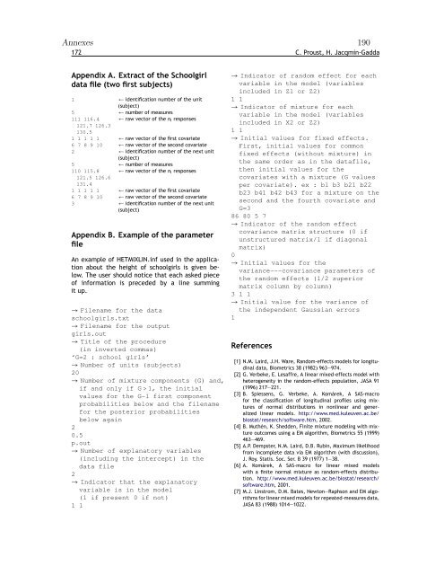
Annexes 190172 C. Proust, H. Jacqmin-GaddaAppendix A. Extract of the Schoolgirldata file (two first subjects)1 ← identification number of the unit(subject)5 ← number of measures111 116.4 ← raw vector of the n i responses121.7 126.3130.51 1 1 1 1 ← raw vector of the first covariate6 7 8 9 10 ← raw vector of the second covariate2 ← identification number of the next unit(subject)5 ← number of measures110 115.8 ← raw vector of the n i responses121.5 126.6131.41 1 1 1 1 ← raw vector of the first covariate6 7 8 9 10 ← raw vector of the second covariate3 ← identification number of the next unit(subject)Appendix B. Example of the parameterfileAn example of HETMIXLIN.inf used in the applicationabout the height of schoolgirls is given below.The user should notice that each asked pieceof information is preceded by a line summingit up.→ Filename for the dataschoolgirls.txt→ Filename for the outputgirls.out→ Title of the procedure(in inverted commas)‘G=2 : school girls’→ Number of units (subjects)20→ Number of mixture components (G) and,if and only if G > 1, the initialvalues for the G-1 first componentprobabilities below and the filenamefor the posterior probabilitiesbelow again20.5p.out→ Number of explanatory variables(including the intercept) in thedata file2→ Indicator that the explanatoryvariable is in the model(1 if present 0 if not)1 1→ Indicator of random effect for eachvariable in the model (variablesincluded in Z1 or Z2)1 1→ Indicator of mixture for eachvariable in the model (variablesincluded in X2 or Z2)1 1→ Initial values for fixed effects.First, initial values for commonfixed effects (without mixture) inthe same order as in the datafile,then initial values for thecovariates with a mixture (G valuesper covariate). ex : b1 b3 b21 b22b23 b41 b42 b43 for a mixture on thesecond and the fourth covariate andG=386 80 5 7→ Indicator of the random effectcovariance matrix structure (0 ifunstructured matrix/1 if diagonalmatrix)0→ Initial values for thevariance---covariance parameters ofthe random effects (1/2 superiormatrix column by column)3 1 1→ Initial value for the variance ofthe independent Gaussian errors1References[1] N.M. Laird, J.H. Ware, Random-effects models for longitudinaldata, Biometrics 38 (1982) 963—974.[2] G. Verbeke, E. Lesaffre, A linear mixed-effects model withheterogeneity in the random-effects population, JASA 91(1996) 217—221.[3] B. Spiessens, G. Verbeke, A. Komárek, A SAS-macrofor the classification of longitudinal profiles using mixturesof normal distributions in nonlinear and generalizedlinear models. http://www.med.kuleuven.ac.be/biostat/research/software.htm, 2002.[4] B. Muthén, K. Shedden, Finite mixture modeling with mixtureoutcomes using a EM algorithm, Biometrics 55 (1999)463—469.[5] A.P. Dempster, N.M. Laird, D.B. Rubin, Maximum likelihoodfrom incomplete data via EM algorithm (with discussion),J. Roy. Statis. Soc. Ser. B 39 (1977) 1—38.[6] A. Komárek, A SAS-macro for linear mixed modelswith a finite normal mixture as random-effects distribution.http://www.med.kuleuven.ac.be/biostat/research/software.htm, 2001.[7] M.J. Linstrom, D.M. Bates, Newton—Raphson and EM algorithmsfor linear mixed models for repeated-measures data,JASA 83 (1988) 1014—1022.