Télécharger le texte intégral - ISPED-Enseignement à distance

More documents

Recommendations

Info

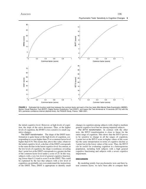
Annexes 196Psychometric Tests’ Sensitivity to Cognitive Changes 5FIGURE 2. Estimated link function (solid line) between the common factor and each of the four tests (Mini-Mental State Examination (MMSE),Benton Visual Retention Test (BVRT), Digital Symbol Substitution Test (DSST), and Isaacs Set Test shortened at 15 seconds (IST15)) with the95% pointwise confidence interval (dashed lines), the PAQUID Study, France, 1989–2001.the initial cognitive level. However, at high levels of cognition,the slope of the curve decreases. Thus, at the higherlevels of cognition, the BVRT is less sensitive to small cognitivechanges.The DSST transformation. The shape of the DSST transformationis quite linear at the high levels of cognition, correspondingto a score higher than 25 or a common factor levelhigher than 0.54. This means that, above this value, whateverthe initial cognitive level, a decline of the DSST correspondsto the same decline in the latent cognitive level. In contrast, atthe low levels of cognition, the shape is nonlinear, revealingthat 1 point lost at the DSST corresponds to a greater declineof the common factor level under a score of 25. In this way,subjects with a very low level of general cognitive functioning(lower than 0.1) tend to score 0 on the DSST. This couldbe explained by the fact that subjects with a low level ofcognition can probably not even understand the instructionsof the DSST. Thus, DSST is appropriate to identify smallchanges in cognition among subjects with a high to mediumgeneral cognitive level but not among impaired subjects.The IST15 transformation. In contrast with the othertests, the IST15 transformation is close to linear for theentire range of cognition. This shows that the IST15 provesto be sensitive to change in all the ranges of cognition;1 point lost at the IST15 score in higher values of the scorehas the same interpretation in terms of cognitive decline as1 point lost in the lower values of the score. Thus, the IST15can be useful for evaluating cognition in a heterogeneouspopulation, including both subjects with a high generalcognitive functioning and subjects with a severe cognitiveimpairment.DISCUSSIONBy modeling jointly four psychometric tests and their latentcommon factor, we have been able to compare their
Annexes 1976 Proust-Lima et al.distributions in all the range of cognition. In this way, weshowed that MMSE and BVRT were not sensitive to cognitivechanges at high levels of cognition and thus were notappropriate to study cognitive aging in prospective studies includinghighly educated people. On the contrary, we showedthat the DSSTwas very sensitive to cognitive changes at highlevels of cognition. However, as it was less sensitive to cognitivechanges at low levels of cognition, it was not suitablefor measuring cognitive changes in heterogeneous populationsconsisting of both highly normal and severely impairedsubjects. In contrast, the IST15 appeared to be a satisfactorycognitive measure in all the range of cognition, which isof substantial interest when studying cognitive aging inpopulation-based cohort studies.The IST15 has several assets when compared with thethree other tests. First, it does not suffer from a floor effector a ceiling effect. Indeed, using cognitive measures withborder effects can lead to misleading results (especially underestimateddeclines) when investigating cognitive changes,since initial scores are often differentially distributed amongexposure groups and the sensitivity of the tests to identifycognitive changes is thus different among these groups (1).Second, the Isaacs Set Test when shortened at 15 seconds,as well as the DSST, includes a speed component that mayexplain its high sensitivity to changes at upper levels of cognition.Indeed, the speed component plays a key role incognitive aging, and it has been shown, for example, thatmost age-related differences in cognition were due to thedecrease in the processing speed (18). Finally, the IST15 is avery brief test, and its instructions are easily understandable.It can therefore be performed in large population-basedstudies even with severely impaired subjects.The methodology we proposed in this paper has severaladvantages that should be discussed. First, the estimated linkfunctions between the test scores and the latent process makeit possible to compare properties of the tests and, especially,their sensitivity to detect cognitive changes within the entirerange of cognition. This is done by modeling jointly variouspsychometric tests for which the hypothesis of a commonfactor is sensible. By the way, it is worth noting that thelatent common factor in this model is actually definedaccording to the pool of psychometric tests used in the analysis.Computing the model with other tests involving differentcognitive components could have an impact on thecommon factor evolution. In this analysis, we used tests thatboth are frequently used and explore different domains ofcognition, because we wanted to select one test for exploringgeneral cognitive decline in heterogeneous populations.The methodology could also be used for selecting sensitivemeasures in a specific domain of cognition. In this case,based on his/her knowledge or on other analyses such asprincipal component analyses, the researcher must choosethe tests that are assumed to measure the same latent cognitiveability in this specific domain and then apply the methodologyto the selected tests.A second asset of the methodology is that, thanks to theestimated transformations of tests, the tests are no longerconstrained to follow a Gaussian distribution as in a standardlinear mixed model. In this way, even if longitudinal evolutionsof the four tests, as presented in figure 1, part B, couldhave actually been estimated using linear mixed models,they would have been obtained under the wrong Gaussianassumption.Finally, as parameters are estimated using the maximumlikelihood estimators, results are robust to data missing atrandom (i.e., when the probability that data are missing doesnot depend on unobserved values given the past observedvalues). Simpler analyses that aim at comparing empiricalmeans of the tests for different age groups are often biased bythe missing data process, especially when the cognitive leveland the dropout are linked, as was previously shown in thePAQUID cohort (17). In this previous work, it was also shownthat the missing at random assumption was probably notstrictly true, but the impact on the estimated evolution wasslight (17, 19). Moreover, even if missing data may blur thecomparison of evolution of the tests’scores, it is very unlikelythat they biased the comparison of test sensitivity, which isthe main objective of this paper. This was checked by comparingtransformations estimated on four subsamples definedby the time of dropout (dropout after the visits at 3, 5, 8, and10 years or complete follow-up) in the spirit of pattern mixtureanalysis (20). Whatever the pattern of dropout, the estimatedtransformations were very similar (results not shown).Some methodological issues of this analysis should, however,be discussed. First, as the results rely on a parametricmodel, adequate fit of the model to the data has been carefullychecked using postfit methods based on the residualsand the predictions developed in Proust et al. (4) (results notshown). An essential part of the model is the link functionbetween the tests and the common factor. The beta cumulativedistribution function was chosen because this transformationwas flexible enough to exhibit very different shapesand depended on only two parameters per test. However,complementary analyses have been performed estimatingthe link functions on a basis of splines instead of the betacumulative distribution functions; they have led to very similarresults while raising more numerical problems due to thelarge number of parameters.Second, in the PAQUID Study, MMSE was the first testfulfilled during each testing session. Consequently, it wasmore frequently completed than the three other tests, particularlyamong impaired subjects. To ensure that test-specificparameters were estimated on the same sample and to maintaincomparability between the tests, we required that everysubject had at least one measure at each test. The 791 subjectsexcluded from the sample were older (median age: 78.6vs. 73.1 years) and less educated (51.5 percent did not graduatefrom primary school vs. 27 percent in the sample) thanthe subjects included in the selected sample, but the range ofthe observed scores was the same. Note also that using longitudinaldata and keeping incident cases of dementia in thesample increased the observed range of cognition and allowedus to compare evolution of each test over time.In conclusion, our results show that the Isaacs Set Testshortened at 15 seconds could be a good candidate to measurecognitive changes in a general population. More generally,the methodology used in this study provides someclues to thoughtfully select the appropriate measures ofcognition collected in a study according to the nature ofthe target population and the objective of the study.
Page 1 and 2:
Université Victor Segalen Bordeaux
Page 3 and 4:
3RemerciementsA Monsieur Jean-Louis
Page 5 and 6:
5Un immense merci à tous ceux que
Page 7 and 8:
7A Delphine et ses mille et une his
Page 9 and 10:
TABLE DES MATIÈRES 92.3.2 Estimati
Page 11 and 12:
TABLE DES MATIÈRES 116.3.1 Adéqua
Page 13 and 14:
Introduction 13ans atteintes d’un
Page 15 and 16:
Introduction 15Mais, pour l’insta
Page 17 and 18:
Introduction 171.2 Problèmes méth
Page 19 and 20:
Introduction 191.2.3 Association en
Page 21 and 22:
Introduction 21QUID suggère que le
Page 23 and 24:
Chapitre 2Etat des connaissancesCe
Page 25 and 26:
Etat des connaissances 25Plusieurs
Page 27 and 28:
Etat des connaissances 27Prise en c
Page 29 and 30:
Etat des connaissances 29Extensions
Page 31 and 32:
Etat des connaissances 31données s
Page 33 and 34:
Etat des connaissances 33variables
Page 35 and 36:
Etat des connaissances 35(2000) ne
Page 37 and 38:
Etat des connaissances 372.3 Modél
Page 39 and 40:
Etat des connaissances 39chapitre 3
Page 41 and 42:
Etat des connaissances 41de mélang
Page 43 and 44:
Etat des connaissances 43Hawkins et
Page 45 and 46:
Etat des connaissances 45tique de d
Page 47 and 48:
Etat des connaissances 47L’estima
Page 49 and 50:
Etat des connaissances 49normales s
Page 51 and 52:
Etat des connaissances 512.4 Modél
Page 53 and 54:
Etat des connaissances 53en tant qu
Page 55 and 56:
Etat des connaissances 55interactio
Page 57 and 58:
Etat des connaissances 57décrite p
Page 59 and 60:
Etat des connaissances 59entre l’
Page 61 and 62:
Etat des connaissances 612.4.3 Cas
Page 63 and 64:
Etat des connaissances 63l’inform
Page 65 and 66:
Modèle nonlinéaire à processus l
Page 67 and 68:
Page 69 and 70:
Page 71 and 72:
Page 73 and 74:
Page 75 and 76:
Page 77 and 78:
Page 79 and 80:
Page 81 and 82:
Page 83 and 84:
Page 85 and 86:
Page 87 and 88:
Page 89 and 90:
Page 91 and 92:
Page 93 and 94:
Chapitre 4Modèle nonlinéaire à c
Page 95 and 96:
Modèle nonlinéaire à classes lat
Page 97 and 98:
Page 99 and 100:
Page 101 and 102:
Page 103 and 104:
Page 105 and 106:
Page 107 and 108:
Page 109 and 110:
Page 111 and 112:
Page 113 and 114:
Page 115 and 116:
Page 117 and 118:
Page 119 and 120:
Page 121 and 122:
Page 123 and 124:
Page 125 and 126:
Page 127 and 128:
Page 129 and 130:
Page 131 and 132:
Page 133 and 134:
Page 135 and 136:
Page 137 and 138:
Page 139 and 140:
Page 141 and 142:
Page 143 and 144:
Page 145 and 146: Modèle nonlinéaire à classes lat
Page 147 and 148: Modèle nonlinéaire à classes lat
Page 149 and 150: Chapitre 6Discussion et perspective
Page 151 and 152: Discussion et perspectives 151la pr
Page 153 and 154: Discussion et perspectives 153Varia
Page 155 and 156: Discussion et perspectives 1556.2 M
Page 157 and 158: Discussion et perspectives 157à cl
Page 160 and 161: Discussion et perspectives 160effet
Page 162 and 163: Discussion et perspectives 162Dans
Page 164 and 165: Chapitre 7BibliographieAmieva, H.,
Page 166 and 167: Bibliographie 1661, S19-25.Brown, E
Page 168 and 169: Bibliographie 168Sons, New-York.Fol
Page 170 and 171: Bibliographie 170Hogan, J. W. et La
Page 172 and 173: Bibliographie 172Lin, H., McCulloch
Page 174 and 175: Bibliographie 174Park, CA.Muthén,
Page 176 and 177: Bibliographie 176Schlattmann, P. (2
Page 178 and 179: Bibliographie 178in the random-effe
Page 180 and 181: Chapitre 8Annexes8.1 Liste des publ
Page 182 and 183: Annexes 182Pau (France)Communicatio
Page 184 and 185: Annexes 184166 C. Proust, H. Jacqmi
Page 192 and 193: AnnexesAmerican Journal of Epidemio
Page 194 and 195: Annexes 194Psychometric Tests’ Se
Page 198 and 199: Annexes 198Psychometric Tests’ Se
Page 200 and 201: Annexes 200Abstract :When investiga
Page 202 and 203: Annexes 202educated subjects. This
Page 204 and 205: Annexes 204(iii) the recognition fo
Page 206 and 207: Annexes 206Explanatory variablesIn
Page 208 and 209: Annexes 208IST15 (median=28, IQR=24
Page 210 and 211: Annexes 210and on the mean evolutio
Page 212 and 213: Annexes 212These findings should be
Page 214 and 215: Annexes 214Appendix : model specifi
Page 216 and 217: Annexes 216References[1] Amieva H,
Page 218 and 219: Annexes 218[19] Letenneur L, Commen
Page 220 and 221: Annexes 220Figure 1 : (A) Predicted
Page 222 and 223: Annexes 222Table 1: demographic and
Page 224: Annexes 224MMSE 0.0037 * 0.0013,0.0
show all

Télécharger le texte intégral - ISPED-Enseignement à distance

Create successful ePaper yourself

Delete template?

Save as template?