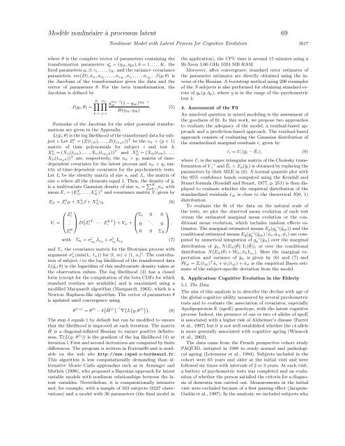
Modè<strong>le</strong> nonlinéaire <strong>à</strong> processus latent 681016 Biometrics, December 2006for the test k; ɛ ijk are independent Gaussian errors with mean0 and variance σ 2 ɛ k.As in Dunson (2003), the random effect α ik accounts for thefact that for a same value of the latent process, two subjectscan score differently in the cognitive domain associated withpsychometric test k. The contrasts γ k make the relationshipbetween the outcomes and the latent process more f<strong>le</strong>xib<strong>le</strong> byallowing some covariates to be differently associated with thevarious outcomes. The sum of the contrasts over the K testsfor a given covariate equals 0. Thus, parameters β in (1) capturethe mean association with the covariates contained bothin X 1i (t) and X 2i (t), whi<strong>le</strong> parameters γ k in (2) capture thevariability of the association for each test around this meanvalue.2.3 The Choice of the Family of Functions GFor all the outcomes, the transformations g k (y; η k ) come fromthe same family of functions G. The choice of the family is akey aspect of the model; it determines the f<strong>le</strong>xibility of thelink between the joint outcomes with various behaviors andthe underlying latent process. The transformations must bemonotonic and increasing functions of y and depend on fewparameters to make the estimation of the model easier. So,the choice of the family G is a compromise between f<strong>le</strong>xibilityand parsimony.The first transformation considered here is the beta cumulativedistribution function (CDF), which can take very differentshapes, including concave, convex, and sigmoid, accordingto the parameters, as illustrated in Figure 1. It is defined fory ∈ [0, 1], η 1k > 0, and η 2k > 0byg k (y; η 1k ,η 2k )=∫ y0x η 1k−1 (1 − x) η 2k−1B(η 1k ,η 2k )dx. (3)As the beta CDF is defined in [0, 1], for each psychometrictest, a preliminary step consists of rescaling the tests to theunit interval.The main drawback of this transformation is its computationalcomp<strong>le</strong>xity. As a consequence, simp<strong>le</strong>r transformationshave also been considered to compare the fits of the models:the linear transformation, the logit transformation combinedwith a linear transformation, and the Weibull cumulative distributionfunction (details in the Appendix). When using alinear transformation, the model is a multivariate linear mixedmodel similar to Roy and Lin (2000) or Rabe-Hesketh et al.(2004), with an additional Brownian motion term. In thatcase, constraints have to be added to make the model identifiab<strong>le</strong>:we assume the intercept μ 0 equals 0 and the variance ofthe random intercept u 0i equals 1. In contrast, when using aCDF, the requirement that g k (y) is in [0, 1] avoids additionalconstraints on the latent process.3. EstimationParameter estimation is achieved using maximum likelihoodtechniques assuming that missing data are missing atrandom. A nonstandard aspect of the model is the presenceof parameters both in the nonlinear transformationg k of the outcome and in the model for the transformedresponse ỹ i =(ỹ i11 ,...,ỹ ini1 1,...,ỹ ijk ,...,ỹ i1K ,...,ỹ iniK K) T ,where ỹ ijk = g k (y ijk ). The log likelihood of interest is the loglikelihood of the outcomes in their natural sca<strong>le</strong>, and thusincludes the Jacobian of the transformations g k . It is given byL(y; θ) =L(ỹ; θ) + ln(J(y; θ))N∑N∑= L(ỹ i ; θ)+ ln(J(y i ; θ)), (4)i=1i=110.8Beta(0.5;2)Beta(3;3)0.6beta(x)0.4Beta(2;0.7)Beta(0.6;0.5)0.200 0.2 0.4 0.6 0.8 1xFigure 1.Examp<strong>le</strong>s of beta transformations for various pairs of parameter values.
Modè<strong>le</strong> nonlinéaire <strong>à</strong> processus latent 69Nonlinear Model with Latent Process for Cognitive Evolution 1017where θ is the comp<strong>le</strong>te vector of parameters containing thetransformation parameters η ′ k =(η 1k,η 2k ),k =1,...,K, thefixed parameters μ, β, γ 1 ,...,γ K , and the variance–covarianceparameters vec(D),σ w ,σ α1 ,...,σ αK ,σ e1 ,...,σ eK . J(y; θ) isthe Jacobian of the transformation given the data and thevector of parameters θ. For the beta transformation, theJacobian is defined byJ(y i ; θ) =n K∏ ∏ ikk=1 j=1y η 1k−1ijk(1 − y ijk ) η 2k−1. (5)B(η 1k ,η 2k )Formulae of the Jacobian for the other potential transformationsare given in the Appendix.L(ỹ i ; θ) is the log likelihood of the transformed data for subjecti. Let Zi k =(Z(t i1k),...,Z(t inik k)) T be the n ik × (p +1)matrix of time polynomials for subject i and test k;X1i k =(X 1i(t i1k ),...,X 1i (t inik k)) T and X2i k =(X 2i(t i1k ),...,X 2i (t inik k)) T are, respectively, the n ik × q 1 matrix of timedependentcovariates for the latent process and n ik × q 2 matrixof time-dependent covariates for the psychometric tests.Let I n be the identity matrix of size n, and J n , the matrix ofsize n where all the e<strong>le</strong>ments equal 1. Then, the density of ỹ iis a multivariate Gaussian density of size n i = ∑ Kn k=1 ik withmean E i =(E T i1 , ..., E iK T )T and covariance matrix V i given byE ik = Zi k μ + X1iβ k + X2iγ k k (6)V i =⎛⎜⎝Z 1 i. .Z K i⎞⎟⎠ D ( Z 1Ti⎛⎞Σ 1 0 0)··· ZiKT ⎜ . + Vw + ⎝ 0 .. ⎟ 0 ⎠ ,0 0 Σ Kwith Σ k = σ 2 α kJ nik + σ 2 ɛ kI nik (7)and V w the covariance matrix for the Brownian process withargument σ 2 w(min(t l , t m )) for (l, m) ∈ [1, n i ] 2 . The contributionof subject i to the log likelihood of the transformed dataL(ỹ i ; θ) is the logarithm of this multivariate density taken atthe observation values. The log likelihood (4) has a closedform (except for the computation of the beta CDFs for whichstandard routines are availab<strong>le</strong>) and is maximized using amodified Marquardt algorithm (Marquardt, 1963), which is aNewton–Raphson-like algorithm. The vector of parameters θis updated until convergence usingθ (l+1) = θ (l) − δ ( ˜H(l) ) −1∇( L( y; θ(l) )) . (8)The step δ equals 1 by default but can be modified to ensurethat the likelihood is improved at each iteration. The matrix˜H is a diagonal-inflated Hessian to ensure positive definiteness.∇(L(y; θ (l) )) is the gradient of the log likelihood (4) atiteration l. First and second derivatives are computed by finitedifferences. The program is written in Fortran90 and is availab<strong>le</strong>on the web site http://www.isped.u-bordeaux2.fr.This algorithm is <strong>le</strong>ss computationally demanding than alternativeMonte Carlo approaches such as in Arminger andMuthén (1998), who proposed a Bayesian approach for latentvariab<strong>le</strong> models with nonlinear relationships between the latentvariab<strong>le</strong>s. Neverthe<strong>le</strong>ss, it is computationally intensiveand, for examp<strong>le</strong>, with a samp<strong>le</strong> of 563 subjects (8227 observations)and a model with 36 parameters (the final model inthe application), the CPU time is around 15 minutes using aBi-Xeon 3.06 GHz 1024 MB RAM.Moreover, after convergence, standard error estimates ofthe parameter estimates are directly obtained using the inverseof the Hessian. A bootstrap method using 200 resamp<strong>le</strong>sof the N subjects is also performed for obtaining standard errorsof g k (y, ˆη k ), where y is in the range of the psychometrictest k.4. Assessment of the FitAn unsolved question in mixed modeling is the assessment ofthe goodness of fit. In this work, we propose two approachesto evaluate the adequacy of the model, a residual-based approachand a prediction-based approach. The residual-basedapproach consists of evaluating the Gaussian distribution ofthe standardized marginal residuals ˆɛ i given byˆɛ i = U i (ỹ i − Êi), (9)where U i is the upper triangular matrix of the Cho<strong>le</strong>sky transformationof V −1iand Êi = E ˆθ(ỹ i ) is obtained by replacing theparameters by their MLE in (6). A normal quanti<strong>le</strong> plot withthe 95% confidence bands computed using the Kendall andStuart formula (Kendall and Stuart, 1977, p. 251) is then displayedto evaluate whether the empirical distribution of thestandardized residuals ˆɛ ijk is close to the theoretical N(0, 1)distribution.To evaluate the fit of the data on the natural sca<strong>le</strong> ofthe tests, we plot the observed mean evolution of each testversus the estimated marginal mean evolution or the conditionalmean evolution, which includes random effects es-−1timates. The marginal estimated means E ˆθ(g k(ỹ ijk )) and the−1conditional estimated means E ˆθ(g k(ỹ ijk ) | û i , ˆα ik , ŵ i ) are computedby numerical integration of g −1k(ỹ ik ) over the marginaldistribution of ỹ ik ,N(E ik (ˆθ); V i (ˆθ)), or over the conditionaldistribution N(E ik (ˆθ)+Ŵik ;ˆσ k I nik ). Here the marginal expectationand variance of ỹ ik is given by (6) and (7) andŴ ijk = Z i (t ijk ) T û i +ŵ i (t ijk )+ˆα ik is the empirical Bayes estimateof the subject-specific deviation from the model.5. Application: Cognitive Evolution in the Elderly5.1 The DataThe aim of this analysis is to describe the decline with age ofthe global cognitive ability measured by several psychometrictests and to evaluate the association of covariates, especiallyApolipoprotein E (apoE) genotype, with the latent cognitiveprocess. Indeed, the presence of one or two ɛ4 al<strong>le</strong><strong>le</strong>s of apoEis associated with a higher risk of Alzheimer’s disease (Farreret al., 1997) but it is not well established whether the ɛ4 al<strong>le</strong><strong>le</strong>is more generally associated with cognitive ageing (Winnocket al., 2002).The data came from the French prospective cohort studyPAQUID, initiated in 1988 to study normal and pathologicalageing (Letenneur et al., 1994). Subjects included in thecohort were 65 years and older at the initial visit and werefollowed six times with intervals of 2 or 3 years. At each visit,a battery of psychometric tests was comp<strong>le</strong>ted and an evaluationof whether the person satisfied the criteria for a diagnosisof dementia was carried out. Measurements at the initialvisit were excluded because of a first passing effect (Jacqmin-Gadda et al., 1997). In the analysis, we included subjects who
- Page 1 and 2:
Université Victor Segalen Bordeaux
- Page 3 and 4:
3RemerciementsA Monsieur Jean-Louis
- Page 5 and 6:
5Un immense merci à tous ceux que
- Page 7 and 8:
7A Delphine et ses mille et une his
- Page 9 and 10:
TABLE DES MATIÈRES 92.3.2 Estimati
- Page 11 and 12:
TABLE DES MATIÈRES 116.3.1 Adéqua
- Page 13 and 14:
Introduction 13ans atteintes d’un
- Page 15 and 16:
Introduction 15Mais, pour l’insta
- Page 17 and 18: Introduction 171.2 Problèmes méth
- Page 19 and 20: Introduction 191.2.3 Association en
- Page 21 and 22: Introduction 21QUID suggère que le
- Page 23 and 24: Chapitre 2Etat des connaissancesCe
- Page 25 and 26: Etat des connaissances 25Plusieurs
- Page 27 and 28: Etat des connaissances 27Prise en c
- Page 29 and 30: Etat des connaissances 29Extensions
- Page 31 and 32: Etat des connaissances 31données s
- Page 33 and 34: Etat des connaissances 33variables
- Page 35 and 36: Etat des connaissances 35(2000) ne
- Page 37 and 38: Etat des connaissances 372.3 Modél
- Page 39 and 40: Etat des connaissances 39chapitre 3
- Page 41 and 42: Etat des connaissances 41de mélang
- Page 43 and 44: Etat des connaissances 43Hawkins et
- Page 45 and 46: Etat des connaissances 45tique de d
- Page 47 and 48: Etat des connaissances 47L’estima
- Page 49 and 50: Etat des connaissances 49normales s
- Page 51 and 52: Etat des connaissances 512.4 Modél
- Page 53 and 54: Etat des connaissances 53en tant qu
- Page 55 and 56: Etat des connaissances 55interactio
- Page 57 and 58: Etat des connaissances 57décrite p
- Page 59 and 60: Etat des connaissances 59entre l’
- Page 61 and 62: Etat des connaissances 612.4.3 Cas
- Page 63 and 64: Etat des connaissances 63l’inform
- Page 65 and 66: Modèle nonlinéaire à processus l
- Page 67: Modèle nonlinéaire à processus l
- Page 71 and 72: Modèle nonlinéaire à processus l
- Page 73 and 74: Modèle nonlinéaire à processus l
- Page 75 and 76: Modèle nonlinéaire à processus l
- Page 77 and 78: Modèle nonlinéaire à processus l
- Page 79 and 80: Modèle nonlinéaire à processus l
- Page 81 and 82: Modèle nonlinéaire à processus l
- Page 83 and 84: Modèle nonlinéaire à processus l
- Page 85 and 86: Modèle nonlinéaire à processus l
- Page 87 and 88: Modèle nonlinéaire à processus l
- Page 89 and 90: Modèle nonlinéaire à processus l
- Page 91 and 92: Modèle nonlinéaire à processus l
- Page 93 and 94: Chapitre 4Modèle nonlinéaire à c
- Page 95 and 96: Modèle nonlinéaire à classes lat
- Page 97 and 98: Modèle nonlinéaire à classes lat
- Page 99 and 100: Modèle nonlinéaire à classes lat
- Page 101 and 102: Modèle nonlinéaire à classes lat
- Page 103 and 104: Modèle nonlinéaire à classes lat
- Page 105 and 106: Modèle nonlinéaire à classes lat
- Page 107 and 108: Modèle nonlinéaire à classes lat
- Page 109 and 110: Modèle nonlinéaire à classes lat
- Page 111 and 112: Modèle nonlinéaire à classes lat
- Page 113 and 114: Modèle nonlinéaire à classes lat
- Page 115 and 116: Modèle nonlinéaire à classes lat
- Page 117 and 118: Modèle nonlinéaire à classes lat
- Page 119 and 120:
Modèle nonlinéaire à classes lat
- Page 121 and 122:
Modèle nonlinéaire à classes lat
- Page 123 and 124:
Modèle nonlinéaire à classes lat
- Page 125 and 126:
Modèle nonlinéaire à classes lat
- Page 127 and 128:
Modèle nonlinéaire à classes lat
- Page 129 and 130:
Modèle nonlinéaire à classes lat
- Page 131 and 132:
Modèle nonlinéaire à classes lat
- Page 133 and 134:
Modèle nonlinéaire à classes lat
- Page 135 and 136:
Modèle nonlinéaire à classes lat
- Page 137 and 138:
Modèle nonlinéaire à classes lat
- Page 139 and 140:
Modèle nonlinéaire à classes lat
- Page 141 and 142:
Modèle nonlinéaire à classes lat
- Page 143 and 144:
Modèle nonlinéaire à classes lat
- Page 145 and 146:
Modèle nonlinéaire à classes lat
- Page 147 and 148:
Modèle nonlinéaire à classes lat
- Page 149 and 150:
Chapitre 6Discussion et perspective
- Page 151 and 152:
Discussion et perspectives 151la pr
- Page 153 and 154:
Discussion et perspectives 153Varia
- Page 155 and 156:
Discussion et perspectives 1556.2 M
- Page 157 and 158:
Discussion et perspectives 157à cl
- Page 160 and 161:
Discussion et perspectives 160effet
- Page 162 and 163:
Discussion et perspectives 162Dans
- Page 164 and 165:
Chapitre 7BibliographieAmieva, H.,
- Page 166 and 167:
Bibliographie 1661, S19-25.Brown, E
- Page 168 and 169:
Bibliographie 168Sons, New-York.Fol
- Page 170 and 171:
Bibliographie 170Hogan, J. W. et La
- Page 172 and 173:
Bibliographie 172Lin, H., McCulloch
- Page 174 and 175:
Bibliographie 174Park, CA.Muthén,
- Page 176 and 177:
Bibliographie 176Schlattmann, P. (2
- Page 178 and 179:
Bibliographie 178in the random-effe
- Page 180 and 181:
Chapitre 8Annexes8.1 Liste des publ
- Page 182 and 183:
Annexes 182Pau (France)Communicatio
- Page 184 and 185:
Annexes 184166 C. Proust, H. Jacqmi
- Page 186 and 187:
Annexes 186168 C. Proust, H. Jacqmi
- Page 188 and 189:
Annexes 188170 C. Proust, H. Jacqmi
- Page 190 and 191:
Annexes 190172 C. Proust, H. Jacqmi
- Page 192 and 193:
AnnexesAmerican Journal of Epidemio
- Page 194 and 195:
Annexes 194Psychometric Tests’ Se
- Page 196 and 197:
Annexes 196Psychometric Tests’ Se
- Page 198 and 199:
Annexes 198Psychometric Tests’ Se
- Page 200 and 201:
Annexes 200Abstract :When investiga
- Page 202 and 203:
Annexes 202educated subjects. This
- Page 204 and 205:
Annexes 204(iii) the recognition fo
- Page 206 and 207:
Annexes 206Explanatory variablesIn
- Page 208 and 209:
Annexes 208IST15 (median=28, IQR=24
- Page 210 and 211:
Annexes 210and on the mean evolutio
- Page 212 and 213:
Annexes 212These findings should be
- Page 214 and 215:
Annexes 214Appendix : model specifi
- Page 216 and 217:
Annexes 216References[1] Amieva H,
- Page 218 and 219:
Annexes 218[19] Letenneur L, Commen
- Page 220 and 221:
Annexes 220Figure 1 : (A) Predicted
- Page 222 and 223:
Annexes 222Table 1: demographic and
- Page 224:
Annexes 224MMSE 0.0037 * 0.0013,0.0