Online proceedings - EDA Publishing Association

II.
MATHEMATICAL MODEL AND NUMERICAL
METHODOLOGY
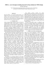
To study Dean Vortex flows with regard to mixing
applications, the geometry of the curved channels and the
schematic diagram of the physical features is expressed in
Fig. 1. The flow system is composed of several staggered
three quarters of ring-shaped channels. The angle between
the lines from the center to two intersections of two
consecutive channels is 90°, and the angle between two lines
of the centers of three consecutive channels is 0°.
11-13
May 2011, Aix-en-Provence, France
channel. For an accelerated convergence, the algebraic
multigrid (AMG) iterative method is applied for pressure
corrections, and the conjugates gradient squared (CGS) and
preconditioning (Pre) solvers are utilized for velocity and
species corrections. The solution is considered converged
when the relative errors of all independent variables are less
than 10 -4 between successive sweeps.
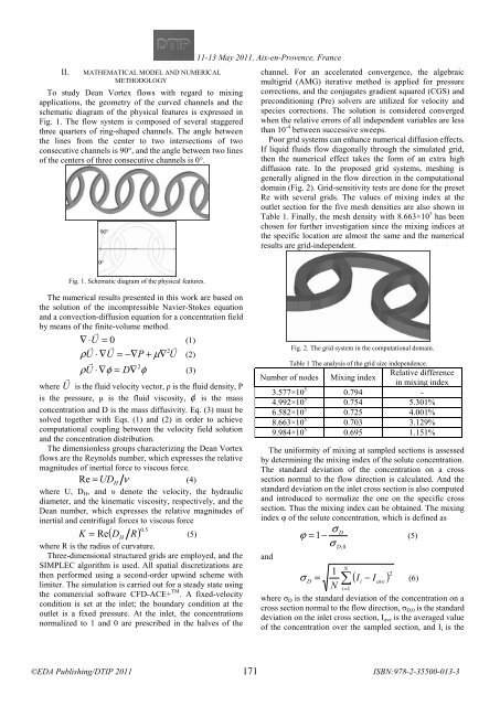
Poor grid systems can enhance numerical diffusion effects.
If liquid fluids flow diagonally through the simulated grid,
then the numerical effect takes the form of an extra high
diffusion rate. In the proposed grid systems, meshing is
generally aligned in the flow direction in the computational
domain (Fig. 2). Grid-sensitivity tests are done for the preset
Re with several grids. The values of mixing index at the
outlet section for the five mesh densities are also shown in
Table 1. Finally, the mesh density with 8.663×10 5 has been
chosen for further investigation since the mixing indices at
the specific location are almost the same and the numerical
results are grid-independent.
Fig. 1. Schematic diagram of the physical features.
The numerical results presented in this work are based on
the solution of the incompressible Navier-Stokes equation
and a convection-diffusion equation for a concentration field
by means of the finite-volume method.
U 0=⋅∇ (1)
−∇=∇⋅
μ
2∇+
UPUU
2
DU
∇=∇⋅
φφρ
(3)
ρ (2)
where U is the fluid velocity vector, ρ is the fluid density, P
is the pressure, μ is the fluid viscosity, φ is the mass
concentration and D is the mass diffusivity. Eq. (3) must be
solved together with Eqs. (1) and (2) in order to achieve
computational coupling between the velocity field solution
and the concentration distribution.
The dimensionless groups characterizing the Dean Vortex
flows are the Reynolds number, which expresses the relative
magnitudes of inertial force to viscous force.
Re = UD H
ν
(4)
where U, D H , and υ denote the velocity, the hydraulic
diameter, and the kinematic viscosity, respectively, and the
Dean number, which expresses the relative magnitudes of
inertial and centrifugal forces to viscous force
= Re
(5)
( ) 5.0
H
RDK
where R is the radius of curvature.
Three-dimensional structured grids are employed, and the
SIMPLEC algorithm is used. All spatial discretizations are
then performed using a second-order upwind scheme with
limiter. The simulation is carried out for a steady state using
the commercial software CFD-ACE+ TM . A fixed-velocity
condition is set at the inlet; the boundary condition at the
outlet is a fixed pressure. At the inlet, the concentrations
normalized to 1 and 0 are prescribed in the halves of the
Number of nodes
Fig. 2. The grid system in the computational domain.
Table 1 The analysis of the grid size independence.
Mixing index
Relative difference
in mixing index
3.577×10 5 0.794 -
4.992×10 5 0.754 5.301%
6.582×10 5 0.725 4.001%
8.663×10 5 0.703 3.129%
9.984×10 5 0.695 1.151%
The uniformity of mixing at sampled sections is assessed
by determining the mixing index of the solute concentration.
The standard deviation of the concentration on a cross
section normal to the flow direction is calculated. And the
standard deviation on the inlet cross section is also computed
and introduced to normalize the one on the specific cross
section. Thus the mixing index can be obtained. The mixing
index φ of the solute concentration, which is defined as
and
σ
D
ϕ 1−= (5)
σ
D 0,
1
σ =
II (6)
D
N
2
∑(
i
−
ave
)
N i=
1
where σ D is the standard deviation of the concentration on a
cross section normal to the flow direction, σ D,0 is the standard
deviation on the inlet cross section, I ave is the averaged value
of the concentration over the sampled section, and I i is the
171