Online proceedings - EDA Publishing Association

A. Quasi-Static response
In order to judge the microphone performance, we need to
estimate the capacity variation ΔC induced by a known
pressure. Supposing that we know the microphone frequency
characteristics, we can do this estimation for DC values. The
estimation of ΔC was done in three approaches. In all of them,
we have compared the microphone capacity without a pressure
with that with a pressure of 1 Pa applied on the diaphragm.
The results obtained in the three cases are shown in Table IV.
For the first approximation, we have used a non-perforated
diaphragm (Fig. 7 (a)) because the electromechanical FEM
simulations of the microphone with a perforated diaphragm
have important computational time requirements, even if
symmetry is assumed and a quarter of the model is simulated.
Based on the predicted value of the pull-in voltage, V PI ,
given by CoventorWare that is between 4.4 V and 4.5 V, we
have decided to use the bias voltage V 0 of 1V. The
corresponding capacitance variation is in Table IV (“FEM”
line)
We can verify these simulation results using an analytic
approach. Indeed, if we consider just the maximum
displacement of the diaphragm, we have the static equation:
2
k mem w max = F pressure + F electrostatic = PA +
ε
00
AV
−
(14)
2
a max
)
And when P = 0 Pa, we have:
max
a
P is the pressure acting on the diaphragm, A is the area of the
diaphragm, V 0 is the bias voltage and B is a correction
coefficient respecting the diaphragm deformation shape
(Fig. 7 (b)). The pull-in effect occurs when the term on the left
side of (15) reaches a maximum:
∂
∂w
max
11-13
May 2011, Aix-en-Provence, France
2
ha
[ B ] =−
0)(
whw
w =
max
When w max = w Pull-in , V
leads to
a max
Pull−in
=
pull
3
8
memhk
a
27ε
BA
0
(16)
− in
3B
(17)
Thanks to (17) and knowing the pull-in voltage by FEM
simulations we can calculate the correction coefficient:
B = 0.385. Once B is calculated, we can solve (14) with the
Cardan method and then calculate the capacitance variation.
Results are summarized in Table IV (“calculation (nonperforated
diaphragm)” line).
simulation. We can see that the calculation and simulation
results are very close. There is a small capacitance deviation is
due to the parasitic capacitance that is taken into account in
the FEM simulation and is not accounted in the analytic
model.
Now, we applied this model for the perforated diaphragm
considering the same value of B that was obtained for the nonperforated
diaphragm. The pull-in voltage is V PI = 4.24 V and
Table IV shows the variation capacitance (“Calculation
(perforated diaphragm)” line).
TABLE IV
CAPACITANCE VARIATION
Approach Conditions w max (nm)
Capacitance
(pF)
FEM
P = 0 Pa
V 0 = 1 V
V 0 = 1 V
53 2.123
P = 1 Pa
133 2.140
V 0 = 1 V
Calculation P = 0 Pa
(nonperforated
51 1.361
P =1 Pa
diaphragm V 0 = 1 V
131 1.378
Calculation
(perforated
diaphragm)
P = 0 Pa
V 0 = 1 V
P = 1 Pa
V 0 = 1 V
57 1.151
147 1.167
ΔC (fF)
(2 B wh
According to the model, the obtained capacitance variation
is very similar as in the non-perforated case. This fact can be
explained either by the estimated value of the correction
2
2 ε
00
AV coefficient B or by a compensation of the decreased stiffness
B
max
)(
=−(15)
whw by a smaller area of a perforated diaphragm.
2kmem
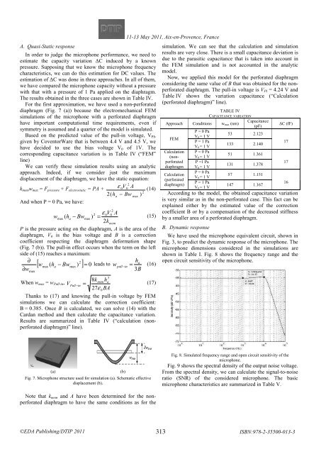
B. Dynamic response
We have used the microphone equivalent circuit, shown in
Fig. 3, to predict the dynamic response of the microphone. The
microphone dimensions considered in the simulations are
shown in Table I. Fig. 8 shows the frequency range and the
open circuit sensitivity of the microphone.
17
17
16
(a)
(b)
Fig. 7. Microphone structure used for simulation (a). Schematic effective
displacement (b).
Fig. 8. Simulated frequency range and open circuit sensitivity of the
microphone.
Fig. 9 shows the spectral density of the output noise voltage.
From the spectral density, we can calculate the signal-to-noise
ratio (SNR) of the considered microphone. The basic
microphone characteristics are summarized in Table V.
Note that k mem and A have been determined for the nonperforated
diaphragm to have the same conditions as for the
©EDA Publishing/DTIP 2011
313