Online proceedings - EDA Publishing Association
Online proceedings - EDA Publishing Association
Online proceedings - EDA Publishing Association

Create successful ePaper yourself
Turn your PDF publications into a flip-book with our unique Google optimized e-Paper software.
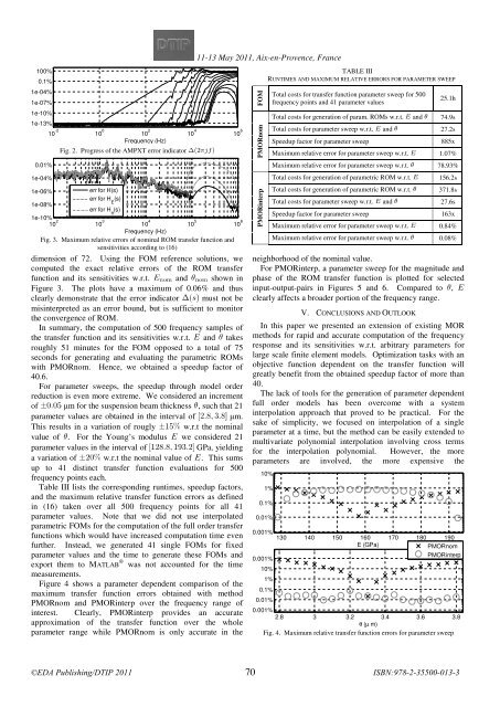
100%<br />
0.1%<br />
1e-04%<br />
1e-07%<br />
1e-10%<br />
1e-13%<br />
10 -2 10 0 10 2 10 4 10 6<br />
Frequency (Hz)<br />
Fig. 2. Progress of the AMPXT error indicator<br />
0.01%<br />
1e-04%<br />
1e-06%<br />
err for H(s)<br />
1e-08%<br />
err for H (s) E<br />
err for H (s) θ<br />
1e-10%<br />
10 2 10 3 10 4 10 5 10 6<br />
Frequency (Hz)<br />
11-13 <br />
May 2011, Aix-en-Provence, France<br />
<br />
TABLE III<br />
RUNTIMES AND MAXIMUM RELATIVE ERRORS FOR PARAMETER SWEEP<br />
Fig. 3. Maximum relative errors of nominal ROM transfer function and<br />
Maximum relative error for parameter sweep w.r.t. 0.08%<br />
sensitivities according to (16)<br />
dimension of 72. Using the FOM reference solutions, we neighborhood of the nominal value.<br />
computed the exact relative errors of the ROM transfer For PMORinterp, a parameter sweep for the magnitude and<br />
function and its sensitivities w.r.t. and shown in phase of the ROM transfer function is plotted for selected<br />
Figure 3. The plots have a maximum of 0.06% and thus input-output-pairs in Figures 5 and 6. Compared to ,<br />
clearly demonstrate that the error indicator must not be clearly affects a broader portion of the frequency range.<br />
misinterpreted as an error bound, but is sufficient to monitor<br />
V. CONCLUSIONS AND OUTLOOK<br />
the convergence of ROM.<br />
In summary, the computation of 500 frequency samples of In this paper we presented an extension of existing MOR<br />
the transfer function and its sensitivities w.r.t. and takes methods for rapid and accurate computation of the frequency<br />
roughly 51 minutes for the FOM opposed to a total of 75 response and its sensitivities w.r.t. arbitrary parameters for<br />
seconds for generating and evaluating the parametric ROMs large scale finite element models. Optimization tasks with an<br />
with PMORnom. Hence, we obtained a speedup factor of objective function dependent on the transfer function will<br />
40.6.<br />
greatly benefit from the obtained speedup factor of more than<br />
For parameter sweeps, the speedup through model order 40.<br />
reduction is even more extreme. We considered an increment The lack of tools for the generation of parameter dependent<br />
of m for the suspension beam thickness , such that 21 full order models has been overcome with a system<br />
parameter values are obtained in the interval of m.<br />
interpolation approach that proved to be practical. For the<br />
sake of simplicity, we focused on interpolation of a single<br />
This results in a variation of rougly w.r.t the nominal<br />
parameter at a time, but the method can be easily extended to<br />
value of . For the Young’s modulus we considered 21<br />
multivariate polynomial interpolation involving cross terms<br />
parameter values in the interval of<br />
GPa, yielding<br />
for the interpolation polynomial. However, the more<br />
a variation of w.r.t the nominal value of . This sums parameters are involved, the more expensive the<br />
up to 41 distinct transfer function evaluations for 500<br />
10%<br />
frequency points each.<br />
Table III lists the corresponding runtimes, speedup factors, 1%<br />
and the maximum relative transfer function errors as defined<br />
in (16) taken over all 500 frequency points for all 41<br />
0.1%<br />
parameter values. Note that we did not use interpolated 0.01%<br />
parametric FOMs for the computation of the full order transfer<br />
0.001%<br />
functions which would have increased computation time even<br />
130 140 150 160 170 180 190<br />
further. Instead, we generated 41 single FOMs for fixed<br />
E (GPa)<br />
PMORnom<br />
parameter values and the time to generate these FOMs and<br />
PMORinterp<br />
export them to MATLAB ®<br />
0.001%<br />
was not accounted for the time<br />
10%<br />
measurements.<br />
1%<br />
Figure 4 shows a parameter dependent comparison of the<br />
0.1%<br />
maximum transfer function errors obtained with method<br />
PMORnom and PMORinterp over the frequency range of<br />
0.01%<br />
0.001%<br />
interest. Clearly, PMORinterp provides an accurate<br />
2.8 3 3.2<br />
approximation of the transfer function over the whole<br />
θ (µ m)<br />
3.4 3.6 3.8<br />
parameter range while PMORnom is only accurate in the Fig. 4. Maximum relative transfer function errors for parameter sweep<br />
FOM<br />
PMORnom<br />
PMORinterp<br />
Total costs for transfer function parameter sweep for 500<br />
frequency points and 41 parameter values<br />
25.1h<br />
Total costs for generation of param. ROMs w.r.t. and 74.9s<br />
Total costs for parameter sweep w.r.t. and 27.2s<br />
Speedup factor for parameter sweep<br />
885x<br />
Maximum relative error for parameter sweep w.r.t. 1.07%<br />
Maximum relative error for parameter sweep w.r.t. 78.93%<br />
Total costs for generation of parametric ROM w.r.t. 156.2s<br />
Total costs for generation of parametric ROM w.r.t. 371.8s<br />
Total costs for parameter sweep w.r.t. and 27.6s<br />
Speedup factor for parameter sweep<br />
163x<br />
Maximum relative error for parameter sweep w.r.t. 0.84%<br />
70