POVERTY REDUCTION STRATEGY TN

decomposition of poverty is done for the year 1999-00. 9 Income level is proxied by mean
consumption expenditure for both rural and urban areas. 10 Fifteen major States in India
were included, which account for about 97 percent of the total population of the country.
Due to differences in the price level, the data are adjusted for price fluctuations by the
using official poverty line.
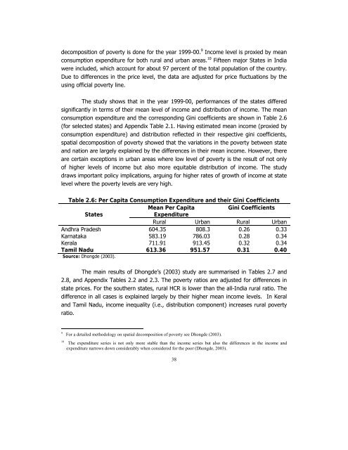
The study shows that in the year 1999-00, performances of the states differed
significantly in terms of their mean level of income and distribution of income. The mean
consumption expenditure and the corresponding Gini coefficients are shown in Table 2.6
(for selected states) and Appendix Table 2.1. Having estimated mean income (proxied by
consumption expenditure) and distribution reflected in their respective gini coefficients,
spatial decomposition of poverty showed that the variations in the poverty between state
and nation are largely explained by the differences in their mean income. However, there
are certain exceptions in urban areas where low level of poverty is the result of not only
of higher levels of income but also more equitable distribution of income. The study
draws important policy implications, arguing for higher rates of growth of income at state
level where the poverty levels are very high.
Table 2.6: Per Capita Consumption Expenditure and their Gini Coefficients
Mean Per Capita
Gini Coefficients
States
Expenditure
Rural Urban Rural Urban
Andhra Pradesh 604.35 808.3 0.26 0.33
Karnataka 583.19 786.03 0.28 0.34
Kerala 711.91 913.45 0.32 0.34
Tamil Nadu 613.36 951.57 0.31 0.40
Source: Dhongde (2003).
The main results of Dhongde’s (2003) study are summarised in Tables 2.7 and
2.8, and Appendix Tables 2.2 and 2.3. The poverty ratios are adjusted for differences in
state prices. For the southern states, rural HCR is lower than the all-India rural ratio. The
difference in all cases is explained largely by their higher mean income levels. In Keral
and Tamil Nadu, income inequality (i.e., distribution component) increases rural poverty
ratio.
9
10
For a detailed methodology on spatial decomposition of poverty see Dhongde (2003).
The expenditure series is not only more stable than the income series but also the differences in the income and
expenditure narrows down considerably when considered for the poor (Dhongde, 2003).
38