Biomechanics and Medicine in Swimming XI
Biomechanics and Medicine in Swimming XI
Biomechanics and Medicine in Swimming XI

Create successful ePaper yourself
Turn your PDF publications into a flip-book with our unique Google optimized e-Paper software.
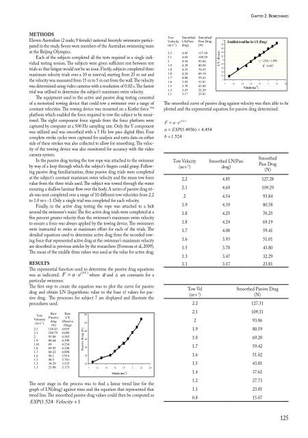
Methods<br />
Eleven Australian (2 male; 9 female) national freestyle swimmers participated<br />
<strong>in</strong> the study. Seven were members of the Australian swimm<strong>in</strong>g team<br />
at the Beij<strong>in</strong>g Olympics.<br />
Each of the subjects completed all the tests required <strong>in</strong> a s<strong>in</strong>gle <strong>in</strong>dividual<br />
test<strong>in</strong>g session. The subjects were given sufficient rest between test<br />
trials so that fatigue would not be an issue. Firstly, subjects completed three<br />
maximum velocity trials over a 10 m <strong>in</strong>terval, start<strong>in</strong>g from 25 m out <strong>and</strong><br />
the velocity was measured from 15 m to 5 m out from the wall. The velocity<br />
was determ<strong>in</strong>ed us<strong>in</strong>g video cameras with a resolution of 0.02 s. The fastest<br />
trial was utilised to determ<strong>in</strong>e the subject’s maximum swim velocity.<br />
The equipment used <strong>in</strong> the active <strong>and</strong> passive drag test<strong>in</strong>g consisted<br />
of a motorised tow<strong>in</strong>g device that could tow a swimmer over a range of<br />
constant velocities. The tow<strong>in</strong>g device was mounted on a Kistler force TM<br />
platform which enabled the force required to tow the subject to be monitored.<br />
The eight component force signals from the force platform were<br />
captured by computer at a 500 Hz sampl<strong>in</strong>g rate. Only the Y component<br />
was utilized <strong>and</strong> was smoothed with a 5 Hz low pass digital filter. Four<br />
complete stroke cycles were captured for analysis <strong>and</strong> extra data on either<br />
side of these strokes was also collected to allow for smooth<strong>in</strong>g. The velocity<br />
of the tow<strong>in</strong>g device was also monitored for accuracy with the video<br />
camera system.<br />
In the passive drag test<strong>in</strong>g the tow rope was attached to the swimmer<br />
by way of a loop through which the subject’s f<strong>in</strong>gers could grasp. Follow<strong>in</strong>g<br />
passive drag familiarization, three passive drag trials were completed<br />
at the subject’s constant maximum swim velocity <strong>and</strong> the mean tow force<br />
value from the three trials used. The subject was towed through the water<br />
ensur<strong>in</strong>g a shallow lam<strong>in</strong>ar flow over the body. A series of passive drag trials<br />
was next completed over a range of 10 different tow velocities from 2.2<br />
to 1.0 m·s -1. Only a s<strong>in</strong>gle trial was completed for each velocity.<br />
F<strong>in</strong>ally, <strong>in</strong> the active drag test<strong>in</strong>g the rope was attached to a belt<br />
around the swimmer’s waist. The five active drag trials were completed at a<br />
five percent greater velocity than the swimmer’s maximum swim velocity<br />
to ensure a force was always applied by the tow<strong>in</strong>g device. The swimmers<br />
were <strong>in</strong>structed to swim at maximum effort for each of the trials. The<br />
detailed equations used to determ<strong>in</strong>e active drag from the recorded tow<strong>in</strong>g<br />
force that represented active drag at the swimmer’s maximum velocity<br />
are described <strong>in</strong> previous articles by the researchers (Formosa et al, 2009).<br />
The mean of the middle three values was used as the value for active drag.<br />
results<br />
The exponential function used to determ<strong>in</strong>e the passive drag equations<br />
( b⋅V<br />
)<br />
was <strong>Biomechanics</strong> as <strong>in</strong>dicated. <strong>and</strong> <strong>Medic<strong>in</strong>e</strong> F = <strong>in</strong> aSwimm<strong>in</strong>g<br />
⋅ e where <strong>XI</strong> Chapter a <strong>and</strong> 2 <strong>Biomechanics</strong> b are constants b for 33 a<br />
particular swimmer.<br />
The first step to create the equation was to plot the curve for passive<br />
The exponential function used to determ<strong>in</strong>e the passive drag equations was as <strong>in</strong>dicated.<br />
drag <strong>and</strong> ( b⋅Vobta<strong>in</strong><br />
) LN (logarithmic value to the base e) values for pas-<br />
F = a ⋅ e where a<strong>and</strong> b are constants for a particular swimmer.<br />
sive The drag. first step The to create processes the equation for was subject to plot 7 the are curve displayed for passive <strong>and</strong> drag <strong>and</strong> illustrate obta<strong>in</strong> LN the<br />
(logarithmic value to the base e) values for passive drag. The processes for subject 7<br />
procedures used.<br />
are displayed <strong>and</strong> illustrate the procedures used.<br />
Tow<br />
Velocity<br />
(m·s -1 )<br />
Raw<br />
Passive<br />
drag<br />
(N)<br />
Raw<br />
LN<br />
(Passive<br />
Drag)<br />
2.2 128.43 4.855<br />
2.1 108.79 4.689<br />
2 95.88 4.563<br />
1.9 80.64 4.390<br />
1.81 69 4.234<br />
1.8 69.95 4.248<br />
1.7 60.22 4.098<br />
1.6 50.1 3.914<br />
1.5 40.5 3.701<br />
1.3 34.29 3.535<br />
1.1 23.88 3.173<br />
P a s s iv e D r a g ( N )<br />
140<br />
120<br />
100<br />
80<br />
60<br />
40<br />
20<br />
1 1.2 1.4 1.6 1.8 2 2.2 2.4<br />
Velocity (m.s -1 )<br />
The next stage <strong>in</strong> the process was to f<strong>in</strong>d a l<strong>in</strong>ear trend l<strong>in</strong>e for the graph of LN(drag)<br />
aga<strong>in</strong>st time <strong>and</strong> the equation that represented that trend l<strong>in</strong>e. The smoothed passive<br />
drag values could then be computed as EXP ( 1.<br />
524 ⋅Velocity + 1.<br />
4936)<br />
Tow<br />
Velocity<br />
(m·s -1 Smoothed Smoothed<br />
LN(Pass Pass Drag<br />
Establish trend l<strong>in</strong>e for LN (Drag)<br />
) drag) (N)<br />
2.2 4.85 127.28<br />
2.1 4.69 109.29<br />
2 4.54 93.84<br />
y = 1.524x + 1.4936<br />
1.9 4.39 80.58<br />
R<br />
1.8 4.25 70.25<br />
1.8 4.24 69.19<br />
1.7 4.08 59.41<br />
2 5<br />
4.8<br />
EXP(<br />
1.<br />
524 ⋅Velocity + 1.<br />
4936 4.6 )<br />
4.4<br />
4.2<br />
4<br />
3.8<br />
= 0.9957<br />
3.6<br />
3.4<br />
3.2<br />
3<br />
The next stage <strong>in</strong> the process was to f<strong>in</strong>d a l<strong>in</strong>ear trend l<strong>in</strong>e for the<br />
graph of LN(drag) aga<strong>in</strong>st time <strong>and</strong> the equation that represented that<br />
trend l<strong>in</strong>e. The smoothed passive drag values could then be computed as<br />
L N (D r a g )<br />
1.6 50.1 3.914<br />
1.5 40.5 3.701<br />
1.3 34.29 3.535<br />
1.1 23.88 3.173<br />
40<br />
20<br />
1 1.2 1.4 1.6 1.8 2 2.2 2.4<br />
chaPter2.<strong>Biomechanics</strong><br />
Velocity (m.s -1 )<br />
The next stage <strong>in</strong> the process was to f<strong>in</strong>d a l<strong>in</strong>ear trend l<strong>in</strong>e for the graph of LN(drag)<br />
aga<strong>in</strong>st time <strong>and</strong> the equation that represented that trend l<strong>in</strong>e. The smoothed passive<br />
drag values could then be computed as EXP ( 1.<br />
524 ⋅Velocity + 1.<br />
4936)<br />
Tow<br />
Velocity<br />
(m·s -1 Smoothed Smoothed<br />
LN(Pass Pass Drag<br />
) drag) (N)<br />
Establish trend l<strong>in</strong>e for LN (Drag)<br />
2.2 4.85 127.28<br />
2.1<br />
2<br />
1.9<br />
1.8<br />
1.8<br />
1.7<br />
1.6<br />
1.5<br />
1.3<br />
4.69<br />
4.54<br />
4.39<br />
4.25<br />
4.24<br />
4.08<br />
3.93<br />
3.78<br />
3.47<br />
109.29<br />
93.84<br />
80.58<br />
70.25<br />
69.19<br />
59.41<br />
51.01<br />
43.80<br />
32.29<br />
y = 1.524x + 1.4936<br />
R<br />
1.1 3.17 23.81<br />
The smoothed curve of passive drag aga<strong>in</strong>st velocity was then able to be plotted <strong>and</strong> the<br />
exponential equation for passive drag determ<strong>in</strong>ed.<br />
( b⋅V<br />
)<br />
F = a ⋅ e<br />
a = EXP(<br />
1.<br />
4936)<br />
= 4.<br />
454<br />
b = 1.<br />
524<br />
2 5<br />
4.8<br />
4.6<br />
4.4<br />
4.2<br />
4<br />
3.8<br />
3.6<br />
3.4<br />
3.2<br />
3<br />
1 1.2<br />
= 0.9957<br />
1.4 1.6 1.8 2 2.2<br />
Velocity (m.s<br />
2.4<br />
-1 )<br />
The smoothed curve of passive drag aga<strong>in</strong>st velocity was then able to be<br />
plotted <strong>and</strong> the exponential equation for passive drag determ<strong>in</strong>ed.<br />
( b⋅V<br />
)<br />
F = a ⋅ e<br />
a = EXP(<br />
1.<br />
4936)<br />
=<br />
b = 1.<br />
524<br />
Tow Velocity<br />
(m·s -1 )<br />
4.<br />
454<br />
L N (D r a g )<br />
Smoothed LN(Pass<br />
drag)<br />
Smoothed<br />
Pass Drag<br />
(N)<br />
2.2 4.85 127.28<br />
2.1 4.69 109.29<br />
2 4.54 93.84<br />
1.9 4.39 80.58<br />
1.8 4.25 70.25<br />
1.8 4.24 69.19<br />
1.7 4.08 59.41<br />
1.6 3.93 51.01<br />
1.5 3.78 43.80<br />
1.3 3.47 32.29<br />
1.1 3.17 23.81<br />
Tow Vel<br />
(m·s -1 )<br />
Smoothed Passive Drag<br />
(N)<br />
2.2 127.31<br />
2.1 109.31<br />
2 93.86<br />
1.9 80.59<br />
1.8 69.20<br />
1.7 59.42<br />
1.6 51.02<br />
1.5 43.81<br />
1.4 37.61<br />
1.2 27.73<br />
1.1 23.81<br />
0.8 15.07<br />
125