Biomechanics and Medicine in Swimming XI

for determination of LT. This study was thus designed to test whether
commonly used analysis techniques were reliable in both test-retest and
analysis-to-analysis comparisons.
Methods
A total of 30 swimmers, female (n=15) and male (n=15) volunteered and
gave their consent to serve as subjects (Table 1). Each subject performed
a standardized pool test of ten 100 meter swims twice in a three-day
period (Gullstrand & Holmer, 1980). Pace-lights were placed linearly
along on the bottom of a 50 meter pool for visually adjusting swimming
velocity. The initial velocity of the exercise was 0.45 m·s -1 less than the
individual maximum velocity. Velocity was increased by 0.05 m·s -1 with
each 100 meter swim until the test ended in exhaustion. The rest interval
between the 100 meter swims was 90 seconds. Time for the 100 meter
swims, as well as for 50 meter laps were taken by hand held watches
to calculate mean velocity. Blood samples (20µl) were taken from the
ear lobe immediately after each swim to obtain BLa (Boehringer-
Mannheim: test-fibel).
Table 1. Physical characteristics of the subjects (mean ± standard deviation).
Age
(years)
Stature
(m)
Body mass
(kg)
BMI
(kg/m 2 )
T100*
(s)
Pooled (n=30) 16.7 ± 3.3 1.70 ± 0.08 61.8 ± 6.6 21.3 ± 1.1 65.2 ± 5.7
Females (n=15) 17.3 ± 3.7 1.68 ± 0.06 60.7 ± 5.9 21.5 ± 1.0 67.3 ± 4.2
Males (n=15) 16.0 ± 2.7 1.72 ± 0.09 62.8 ± 7.1 21.2 ± 1.1 62.8 ± 6.3
*Time for best personal performance in 100 meter freestyle swimming
Two experienced analysts were used to define the LT from each test. The
results from the analyses were compared between the two analysts. The
BLa-velocity graphs were plotted, and subsequently the four different
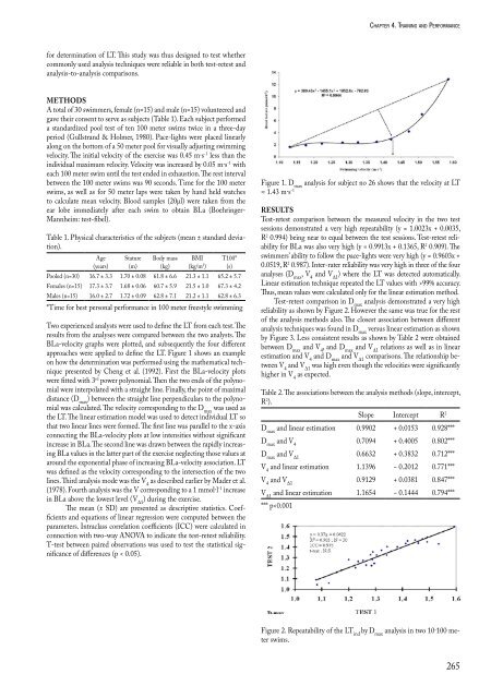
approaches were applied to define the LT. Figure 1 shows an example
on how the determination was performed using the mathematical technique
presented by Cheng et al. (1992). First the BLa-velocity plots
were fitted with 3 rd power polynomial. Then the two ends of the polynomial
were interpolated with a straight line. Finally, the point of maximal
distance (D max ) between the straight line perpendiculars to the polynomial
was calculated. The velocity corresponding to the D max was used as
the LT. The linear estimation model was used to detect individual LT so
that two linear lines were formed. The first line was parallel to the x-axis
connecting the BLa-velocity plots at low intensities without significant
increase in BLa. The second line was drawn between the rapidly increasing
BLa values in the latter part of the exercise neglecting those values at
around the exponential phase of increasing BLa-velocity association. LT
was defined as the velocity corresponding to the intersection of the two
lines. Third analysis mode was the V 4 as described earlier by Mader et al.
(1978). Fourth analysis was the V corresponding to a 1 mmol·l -1 increase
in BLa above the lowest level (V ∆1 ) during the exercise.
The mean (± SD) are presented as descriptive statistics. Coefficients
and equations of linear regression were computed between the
parameters. Intraclass correlation coefficients (ICC) were calculated in
connection with two-way ANOVA to indicate the test-retest reliability.
T-test between paired observations was used to test the statistical significance
of differences (p < 0.05).
chaPter4.trainingandPerformance
Figure 1. D max analysis for subject no 26 shows that the velocity at LT
≈ 1.43 m·s -1
results
Test-retest comparison between the measured velocity in the two test
sessions demonstrated a very high repeatability (y = 1.0023x + 0.0035,
R 2 0.994) being near to equal between the test sessions. Test-retest reliability
for BLa was also very high (y = 0.9913x + 0.1365, R 2 0.909). The
swimmers’ ability to follow the pace-lights were very high (y = 0.9603x +
0.0519, R 2 0.987). Inter-rater reliability was very high in three of the four
analyses (D max , V 4 and V ∆1 ) where the LT was detected automatically.
Linear estimation technique repeated the LT values with >99% accuracy.
Thus, mean values were calculated only for the linear estimation method.
Test-retest comparison in D max analysis demonstrated a very high
reliability as shown by Figure 2. However the same was true for the rest
of the analysis methods also. The closest association between different
analysis techniques was found in D max versus linear estimation as shown
by Figure 3. Less consistent results as shown by Table 2 were obtained
between D max and V 4 , and D max and V ∆1 relations as well as in linear
estimation and V 4 and D max and V ∆1 comparisons. The relationship between
V 4 and V ∆1 was high even though the velocities were significantly
higher in V 4 as expected.
Table 2. The associations between the analysis methods (slope, intercept,
R2 ).
Slope Intercept R2 Biomechanics and Medicine in Swimming XI / Chapter 4 Training
Dmax and linear estimation 0.9902 + 0.0153 0.928***
Dmax Dmax and Vlinear 4 estimation 0.9902 0.7094 + 0.0153 + 0.4005 0.928*** 0.802***
Dmax D and V4
max and V∆1 Dmax and VΔ1
V4 V4 and linear estimation
0.7094 0.6632
0.6632
1.1396 1.1396
+ 0.4005 + 0.3832 0.802*** 0.712***
+ 0.3832 0.712***
− 0.2012 − 0.2012 0.771*** 0.771***
V4 V4 and VΔ1 V∆1 VΔ1 and linear estimation
*** V∆1 and p